
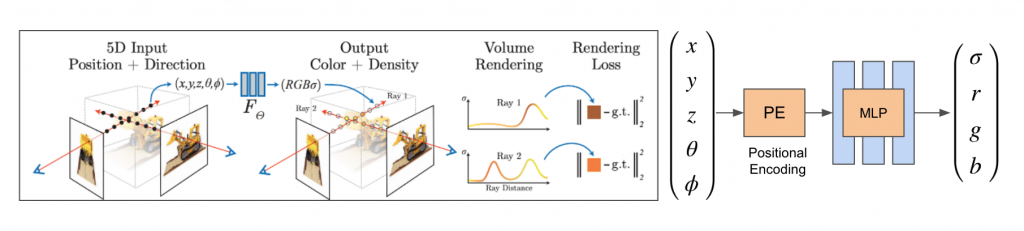
The scene is encoded as a continuous function with a 5-dimensional input of 3D (x, y, z) coordinates and view direction (2 dimensions). For each 3D point, we predict (r, g, b) color and a density value. The 5D input is encoded using positional encoding and given as input to an MLP.
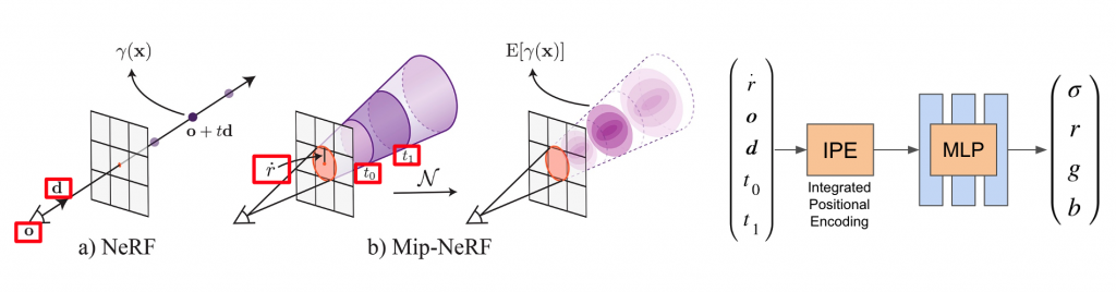
Mip-NeRF
While the original NeRF paper traces rays through the world, we leverage the physically-grounded thin lens model where each pixel on the image sensor observes a cone of light through the lens. By leveraging prior work (Mip-NeRF) that predicts a color (r, g, b) and density values for each section (conical frustum) of this cone, we apply similar concepts for our formulation.
Our Approach
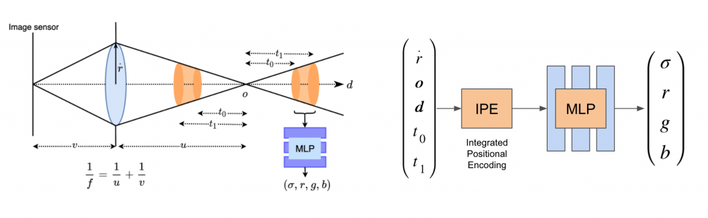
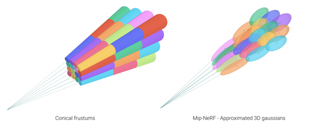
We sketch out the cones that are formed for each pixel of the image sensor. Each cone is divided into smaller conical frustums approximated as 3D spherical Gaussians. The mean and variance of each gaussian are computed and encoded using an integrated positional encoding mechanism. An MLP uses this encoded input to predict color and density. The color for each pixel is the transmittance for the cone of light that each pixel sees.
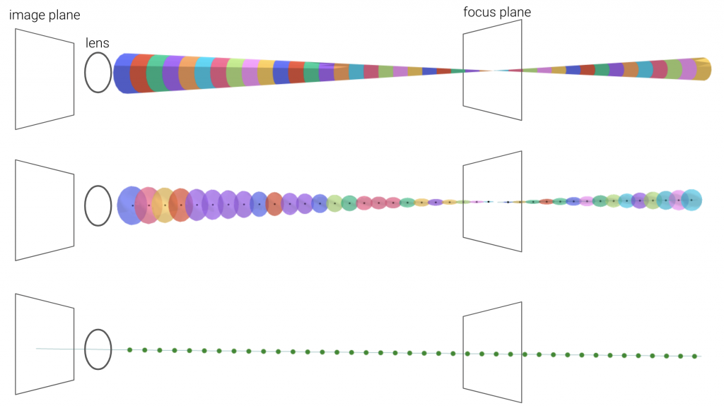
Middle row: 3D spherical Gaussians approximating the conical frustums.
Bottom row: Mean of each 3D Gaussian which are encoded and passed as input to the network
Synthetic Datasets

Experiments on Small Scene Dataset
1. Single Stack Training
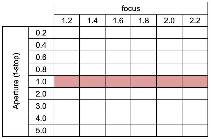
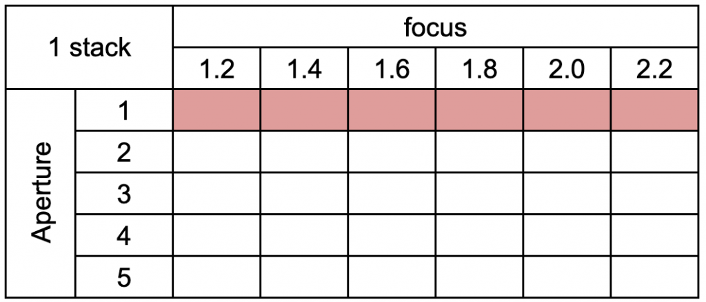
We train the network for a single focal stack as shown in red in the table above. The focus point ranges from the closest tip of the Lego Bulldozer to the furthest tip. The visualization of the training focal stack is shown in the image in the top right.
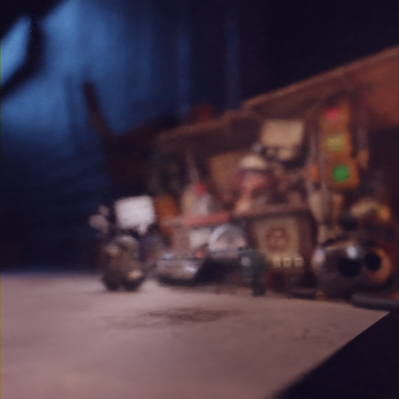
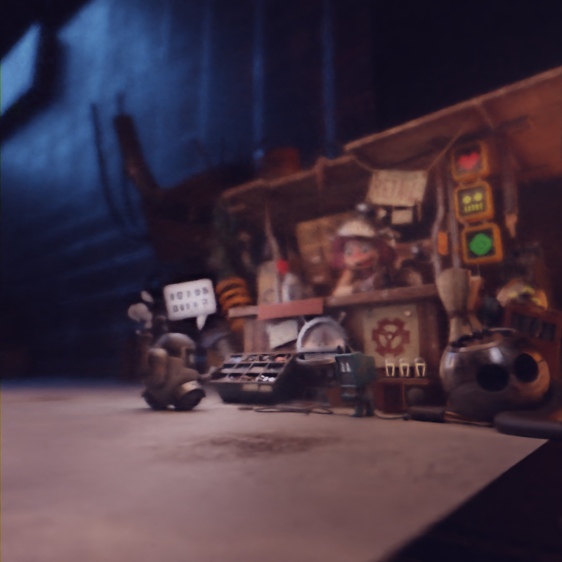
Rendering All-In-Focus (AIF) Image
We render an All-In-Focus image and compare it to the corresponding ground-truth image as shown in the animation above. Closely observing the rendered image showcases blurry artifacts near the center of the image. This indicates that the network does not infer the depth of that region correctly hence producing artifacts. This can be overcome by providing training images with more than one aperture value as shown in the following sub-section.
FOCUS INTERPOLATION
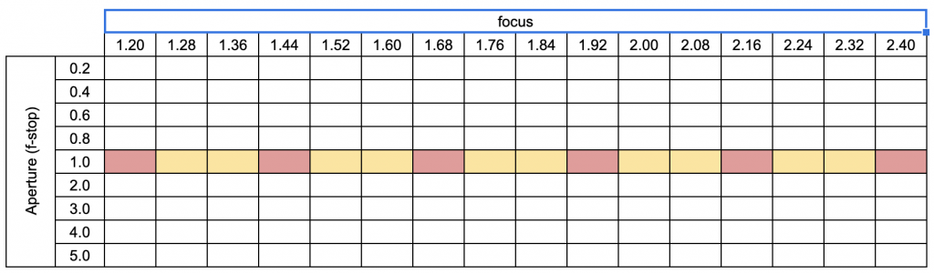

We evaluate our network on focus points in between the training focus points. The training focal points are shown in red while the evaluation focus points are shown in yellow in the table above. The sweep of the entire focus range is shown in the GIF above. We observe a smooth sweep of the images indicating that the network learns a consistent depth representation of the scene.
APERTURE EXTRAPOLATION
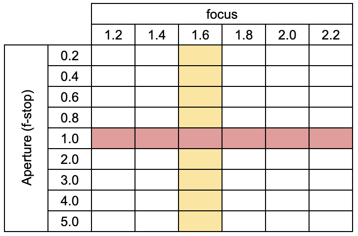

We evaluate our approach on an aperture stack as shown in yellow while the training images are shown in red. The aperture sweep of the rendered images is shown above with the focus plane on the bulldozer blade. Again, we observe a very smooth interpolation of images for the entire aperture sweep showing that the network is able to learn a consistent scene depth representation from a single training focus stack.
2. Multi-Stack Training
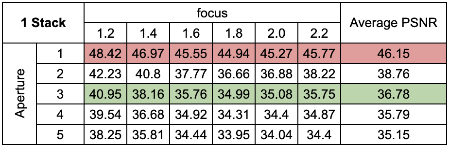
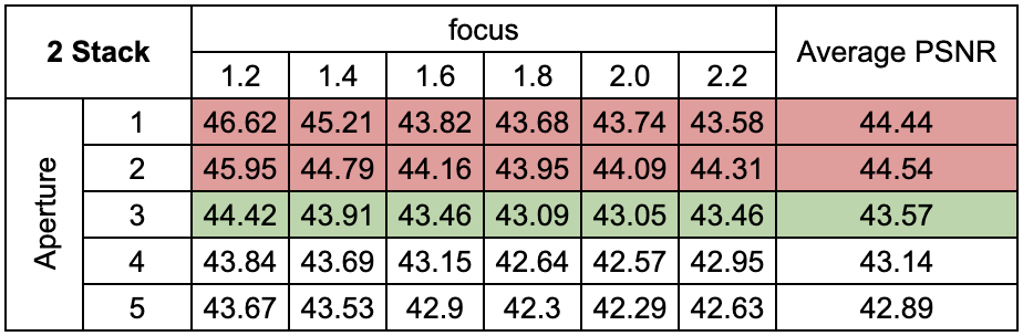
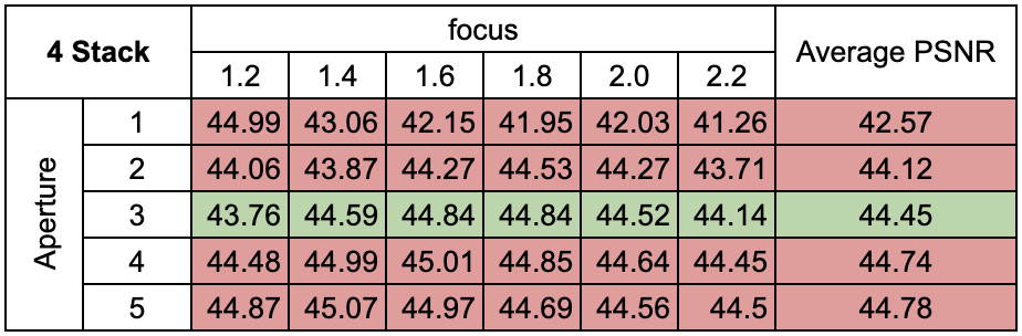
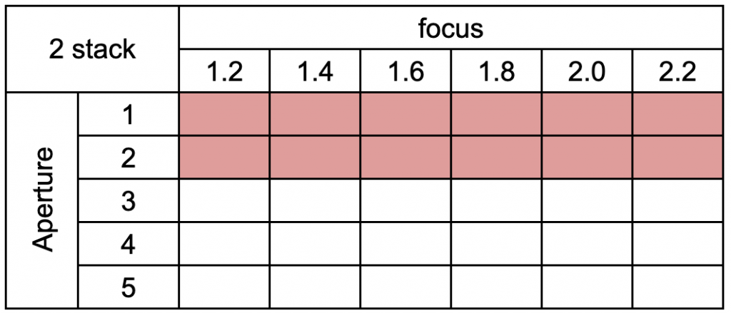
We evaluate the effect of training multiple focal stacks on the test set PSNR. The third focal stack (shown in green) is kept as the test set while the red images are part of the training set. We observe that increasing the number of training focus stacks from 1 to 2 improves the test PSNR by a huge margin. A minimal increase in metrics is observed when increasing the number of training stacks from 2 to 4.
We conclude that a decent performance can be achieved if the number of training images includes varied focus-aperture pairs. Hence a suitable sampling strategy is investigated in the sub-section below.
3. Sampling Strategy
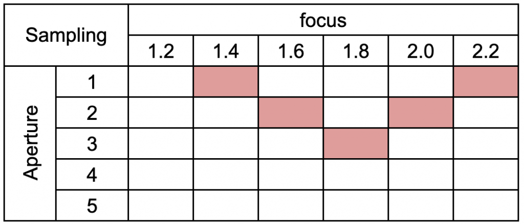
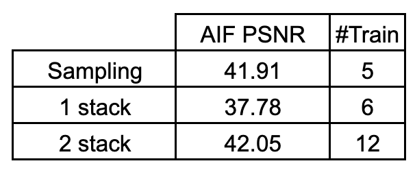
We investigate the effect of randomly sampling the Focus-Aperture grid for generating the training images. The random sampling strategy is shown on the top row, right image. We compare the All-In-Focus image PSNR with that of the single stack and two stack training experiments. We observe that randomly sampling the training images gives very competitive metrics; even better than that of two-stack training. This indicates that providing images from a diverse range of focus-aperture values gives the network the most amount of information that can be exploited to learn a consistent scene-depth representation.
Experiments on Large Scene


We showcase results for rendering an All-In-Focus image (AIF) trained on a varied number of focus stacks for the large scene dataset above. We infer that with an increase in the number of training focus stacks, the image quality improves but still suffers from major blurry artifacts. We conclude that this is caused due to the inability of the network to learn the large range of scene depths from a few ray sample points.
Experiments on Real Dataset
We train our network on a real focus-aperture dataset. The dataset contains 45 focus points and 18 f-stop numbers of which we use two focal stacks as the training set. We render images with a focus point in the center of the scene with varying f-stop numbers i.e. we generate an aperture sweep with the focus at the scene mid-point.
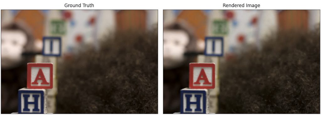
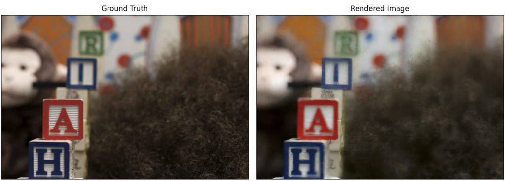
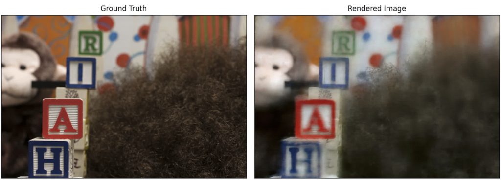
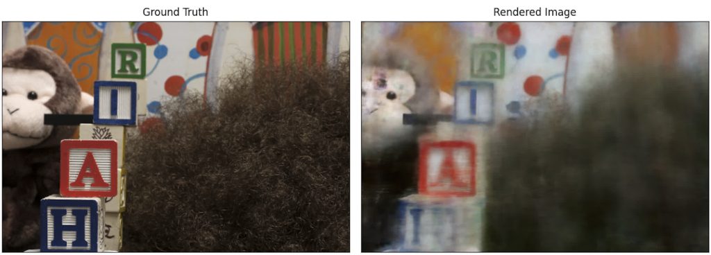
We can observe that the training images (first two rows) are rendered close to ground truth. For the remaining rendered images, the network has to learn to extrapolate. We observe with increasing f-stop numbers, the network generates worse results. This can be attributed to the missing camera calibration parameters in the dataset which leads to incorrect camera modeling.