Related Work:
2DPASS: 2D Priors Assisted Semantic Segmentation on LiDAR Point Clouds
In autonomous driving, cameras provide dense color information and fine-grained texture, but they are quite unreliable in low light conditions. LiDARs could offer accurate and wide-ranging depth information regardless of lighting variances but only capture sparse and textureless data. As camera and LiDAR sensors capture complementary information, it would be essential to conduct semantic segmentation through multi-modality data fusion. Existing fusion-based approaches require paired input data in both training and inference stages, which is not practical in most cases due to the difference of field of views between cameras and LiDars. It’s computational cost is also high as fusion-based models process both images and point clouds at runtime. A general training scheme was introduced as 2DPASS, by leveraging a multi-scale auxiliary modal fusion and knowledge distillation, to acquire richer semantic and structural information from the multimodal data.
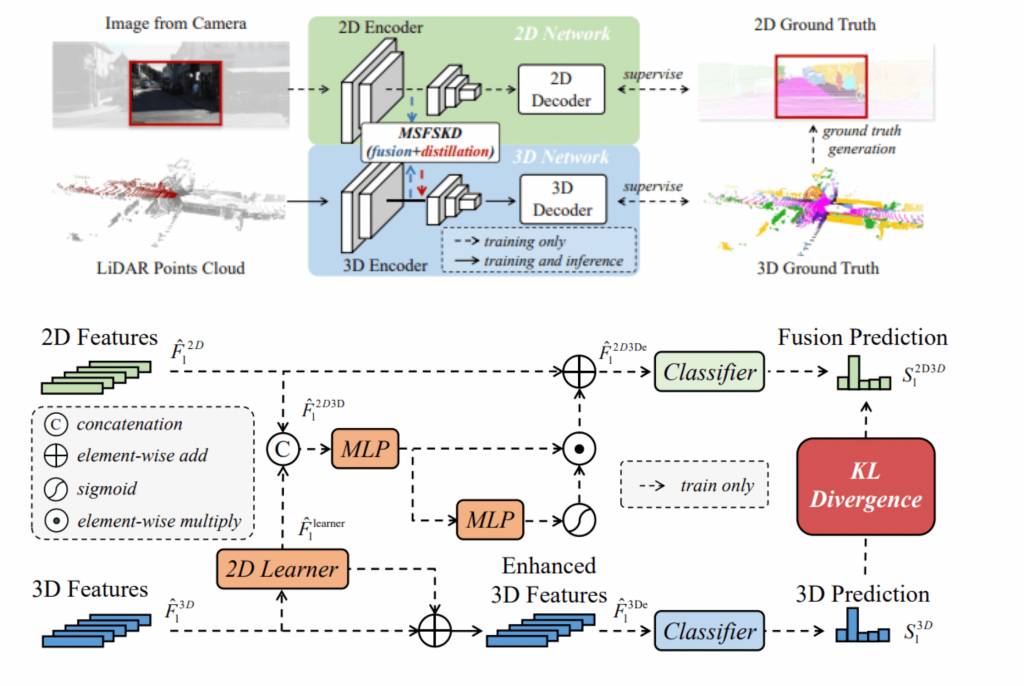
The upper part is the general model. It first crops a small patch from the original camera image as the 2D input. Then the cropped image patch and LiDAR point cloud pass through the 2D and 3D encoders independently to generate multi-scale features. For each scale, we go through this MSFSKD which stands for multi-scale fusion-tosingle knowledge distillation process which is shown here. The modality fusion is first adopted to enhance multi-modality feature. And then, the enhanced feature promotes the 3D representation through the uni-directional Modality-Preserving KD to get the 3D Predictions. And after this part, the feature maps are used to generate the final semantic scores using modal-specific decoders, which are supervised by pure 3D labels.
Cross-modal Learning for Domain Adaptation in 3D Semantic Segmentation
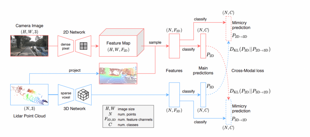
The cross-modal learning for domain adaptation paper was the inspiration of the 2DPASS method. The same as the 2DPASS paper, the cross-modal learning framework also aims to take advantage of the domain gap differences between cameras and Lidars. In their model, a 2D and a 3D network take an image and a point cloud as inputs respectively and predict their own 3D segmentation labels, during which process the 2D predictions are uplifted to 3D. And then the crossmodal learning enforces consistency between the 2D and 3D predictions via mutual mimicking, which is beneficial for domain adaptation in both unsupervised and semi-supervised learning. And that leads to the main topic of this paper, is to constrain the network to make correct predictions on labeled data and consistent predictions across modalities on unlabeled target-domain data, which closely aligns our project that aims to give accurate segmentations on the rare conditions that may not exist in the training dataset.
The below part is the architecture of the method. There are two independent network streams: a 2D stream (in red) which takes an image as input and uses a U-Net-style 2D ConvNet, as well as a 3D stream (in blue) which takes a point cloud as input and uses a U-Net-Style 3D SparseConvNet. Then, the 3D points that have labels are projected into the image and the 2D features are sampled at the corresponding pixel locations. The four segmentation outputs consist of the main predictions and the 2D mimicry predictions, which are transferred across modalities using KL divergences to use the 2D mimicry prediction to estimate the main 3D prediction.
Methods and Experiments
Initial Approach:
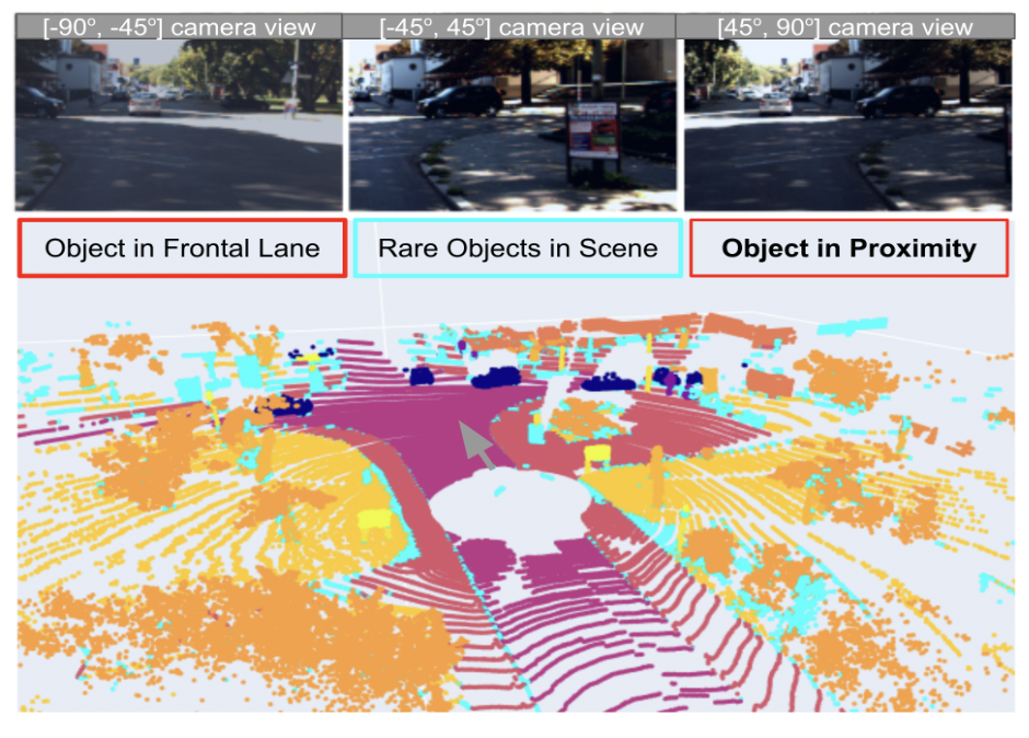
Before a car can recognize any objects that are not labeled, we start with manual definitions of “Road Conditions” (RCs) that categorize the surrounding environment in the driving scenarios. These road conditions can be annotated at the frame level, making it possible for a deep learning model to learn and inference. Thanks to the rich development experience from Honda 99P Labs, we defined three specific RCs:
- Object in Frontal Lane: Recognizing and segmenting objects that are directly in front of the vehicle in its trajectory.
- Rare Objects in the Scene: Identifying and differentiating objects that seldom appear in the dataset or real-world driving scenarios.
- Object in Proximity: Detecting and cataloging objects based on their closeness to the vehicle, essential for immediate response scenarios.
To annotate these RCs, our methodology is to select rare scenes based on high/low confidence scores and improve the SOTA (2DPASS[1] )model on the SemanticKITTI dataset for semantic segmentation. We performed frame-wise RC identification and localization by point-level semantic segmentation and object-level detection. Improved robustness of known points and objects and also parsed unknown points and objects.

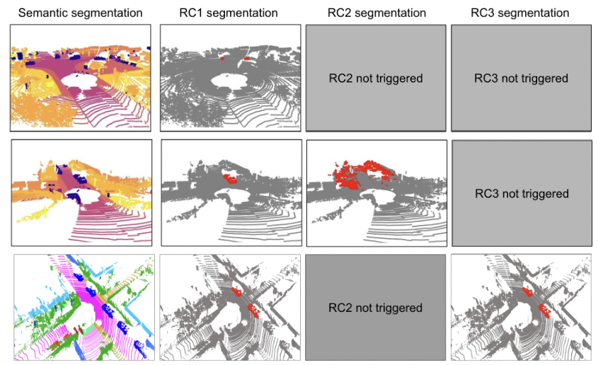
Initial Results: Our preliminary results for mapping the lidar points to RCs are in the table below. The RC1 and RC3 that involve frequently-apppearing objects can be identified and localized, while RC2 that involves rare objects can be identified by cannot be localized. This is straightforward for a machine learning system that is biased by the imbalanced training data distribution. Moreover, the dependency of training data distribution will pose a bigger challenge for unknown objects that never appear in the training data.

Remaining Challenges: The initial results above unveiled two persistent issues to be addressed for reliable scene understanding:
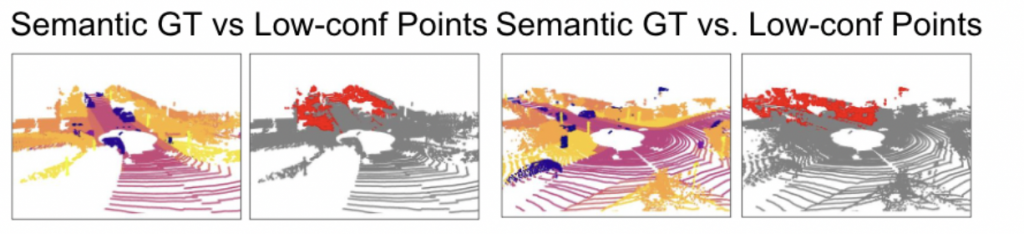
- Missing rare object detections: The online-predicted low-confidence points (points where the system wasn’t sure of its prediction) were misaligned with offline-trained low-metric classes, suggesting a discrepancy in our defined rare objects and the real rare objects on road. For instance, the table below highlights the offline-trained low-metric classes in orange on the Semantic KITTI dataset. The images below show a frame with the rare road condition, which is identified when the frame-wise low confidence(<0.5) lidar points is 30% or more over all the lidar points.

- Incorrect high confidence detections: Objects or object parts may be incorrectly detected as other known objects with high confidence. In the example image below, a cat is detected as two pedestrains with high confidence.

Both these issues can be traced back to the lack of balanced training data over classes. In particular, the public databases in autonomous driving scenarios do not contain unexpected objects on the road. These issues on rare object detection hinder our ability to identify and localize rare/unexpected road conditions.
Large-Language-Model Approach:
To overcome the challenges above, we shift to leverage the Large Language Models (LLMs) for their ability to recognize and describe open-vocabulary objects. This allows us to build a new pipeline to identify and assess the danger level of unexpected road conditions involving both expected and unexpected objects.
As the diagram in below figure suggests, we first apply the Grounded SAM model[2] to produce object instance segmentation given the text prompts. The segmented object instances are then sent to the LENs model[3] for object-level attribute description. Finally, we generate a comprehensive description of road conditions with object-level categories, location, attributes, and danger levels. We hope this pipeline presents the cars with rich information to understand road conditions and adjust driving strategies.

The LENs model can process an image patch of a single object instance with three modules:
- Tag Module: Using a contrastive model, the Tag Module categorizes objects and scene elements with specific tags. For instance, in the given image, it has identified tags like “Mercedes benz sls amg”, “Toy vehicle”, and “Model car”.
- Attribute Module: This module further refines the categorization by attributing specific features or characteristics to the identified objects. Using its attribute vocabulary and contrastive model, it can define an object like a toy car with attributes such as “motor vehicle which has metal or plastic body”.
- Image Captioning Module: Beyond tags and attributes, the system can generate descriptive captions for the scene. It does this by analyzing the input image and generating relevant captions, like “a small car with white trim and wheels on the street” or “a red toy car with an umbrella over the side of the road”.
Thanks to the LENs modules, we are able to generate rich attribute descriptions for the objects that are not annotated in the training dataset. At the output of our pipeline, we reach a rule-based dangerous level assessment like the following example:
- Define Rule Set:
- Rule 1: If the object’s size is large and its speed is high, assign a high dangerous level.
- Rule 2: If the object’s size is medium and its speed is moderate, and it is located in the path of the vehicle, assign a high danger level.
- Rule 3: If the object’s size is small and its speed is low, assign a medium dangerous level.
- Rule 4: If the object is located in the blind spot of the vehicle, assign a medium dangerous level.
- Rule 5: If the object’s behavior is erratic or unpredictable, assign a high dangerous level.
- Rule 6: If the object is made of a hazardous material or has a composition that poses additional risks, assign a higher dangerous level.
- Rule 7: If the object is in poor weather conditions (e.g., heavy rain, fog, snow), assign a higher dangerous level.
- Rule 8: If the object is on a slippery or hazardous road surface (e.g., ice, gravel, potholes), assign a higher dangerous level.
- Inputs:
- Object size (e.g., small, medium, large)
- Object speed (e.g., low, moderate, high)
- Object location (e.g., in path, blind spot)
- Object behavior (e.g., predictable, erratic)
- Object material (e.g., hazardous, non-hazardous)
- Object composition (e.g., fragile, explosive, stable)
- Weather conditions (e.g., rain, fog, snow)
- Road conditions (e.g., slippery, hazardous)
- Rule Evaluation:
- Evaluate each rule based on the inputs and determine if they are satisfied.
- Output:
- Assign a dangerous level based on the rules and their respective priorities. For example, a high dangerous level if Rule 1 or Rule 2 or Rule 6 or Rule 7 or Rule 8 is satisfied, a medium dangerous level if Rule 3 or Rule 4 is satisfied, and so on.
Alternatively, we also integrate LLM (GPT-4) to extrapolate the danger levels of road conditions based on the object attributes. In the toy car example above, we produce the following assessment:
- Physical Damage:
- Toy Car: Given that the toy car is small and lightweight, it’s unlikely to cause significant physical damage to an autonomous vehicle. Running over a toy car would generally not harm the vehicle’s mechanics, tires, or undercarriage.
- Danger Score: 2 out of 10
- Obstruction:
- Toy Car: An autonomous vehicle’s sensors and cameras are designed to detect obstacles, including small ones. A toy car on the road could be detected as an obstruction. While the vehicle might be able to drive over it without harm, the autonomous vehicle’s system might choose to stop or swerve to avoid it. The latter can be especially problematic if the vehicle swerves into an occupied lane or off the road.
- Danger Score: 6 out of 10
- Secondary Dangers:
- Toy Car: Secondary dangers refer to the potential hazards that arise as a consequence of the primary obstruction. If an autonomous vehicle stops or swerves to avoid the toy car, it could result in unexpected behavior that might confuse other drivers, potentially leading to accidents. Furthermore, human drivers might not anticipate the actions of the autonomous vehicle, leading to further complications.
- Danger Score: 7 out of 10
Overall Danger Level: Given the scores in each category, we can average them for an overall danger rating: (2 + 6 + 7) ÷ 3 = 5
Overall, the danger level of a toy car sitting on the street to an autonomous vehicle is 5 out of 10. It’s essential to note that the actual danger level can vary based on the specific situation, type of autonomous vehicle, environmental conditions, and other factors.
Result: Danger Level: 5/10 (Physical Damage: 2, Obstruction: 6, Secondary Dangers: 7)
Notably, at the end of this capstone project (Nov. 2023), ChatGPT also supported image inputs and could output text describing the rare objects on the road. However, ChatGPT’s result is only a sense-based description without precise localization and segmentation of the objects. Therefore it could not trace back the objects responsible for the scene description, and cannot be used to help with autonomous vehicle’s decision-making and route planning.
Conclusion:
With LLM models integrated, we reach a two-pronged road condition understanding: Firstly, recognizing the open-vocabulary object and its attributes, and Secondly, assessing its potential danger quotient at the scene level. These danger levels, subsequently, were tagged with additional object features. This integration became crucial, especially for real-world applications, as it provided an understanding of not just ‘what’ is on the road, but also ‘how dangerous’ it might be. When road conditions occur, we can also trace back to the object that is causing the road conditions. Overall, with these methods and experiments, we initiated a comprehensive and dynamic semantic segmentation tool that not only identifies and segments objects but also understands their potential implications on road safety.
Reference:
- Yan, X., Gao, J., Zheng, C., Zheng, C., Zhang, R., Cui, S., Li, Z.: 2DPASS: 2D Priors Assisted Semantic Segmentation on LiDAR Point Clouds. In: arXiv (2022) arXiv:2207.04397.
- Liu, S., Zeng, Z., Ren, T., Li, F., Zhang, H., Yang, J., Li, C., Yang, J., Su, H., Zhu, J., et al.: Grounding DINO: Marrying DINO with Grounded Pre-training for Open-set Object Detection. In: arXiv preprint (2023) arXiv:2303.05499.
- Berrios, W., Mittal, G., Thrush, T., Kiela, D., Singh, A.: Towards Language Models That Can See: Computer Vision Through the LENS of Natural Language. In: arXiv (2023) arXiv:2306.16410.