See Introduction for a description of the background and rationale behind these updates.
EnvelopeNet
In the classical pipeline, we first compute envelope images from by squaring, averaging, and subtracting the input image stack. This process leaves us with the equivalent of the input images to PSI, without the carrier-wave oscillations.
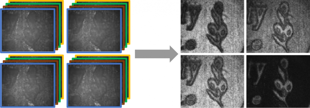
Denoising in the process occurs at this stage: either a Gaussian filter or a bilateral filter conditioned on the RGB image is applied to the envelope images, smoothing them out.
However, this approach discards what may be useful correlations between nearby pixels in the captured frames. We aim to demonstrate a CNN that is capable of learning a more robust envelope extraction function before correlations are removed by denoising. This work is in progress.
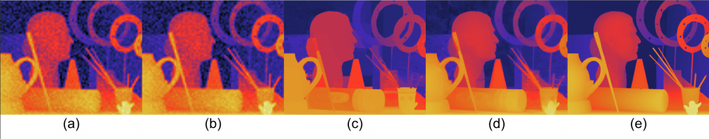
Simulating SWI Frames
In order to train EnvelopeNet, we need a large number of diverse scenes with ground-truth depth and realistic SWI image stacks. Unfortunately, OCT is a time-consuming process (on the order of hours per scene), which means that it is not feasible to create a real training dataset. We address this problem by creating a SWI simulator that generates an SWI image stack based on an input depth map.
To demonstrate the correctness of the SWI simulator, we provide it the OCT depth map of a test scene, then take the simulated frames and run it through the classical pipeline. Theoretically, this is a round-trip operation and should provide us similar results to that of the pipeline run on the real SWI input frames.
To generate a sufficiently large dataset, we apply the SWI simulator to the vast trove of ground-truth images available in the Hypersim Dataset.
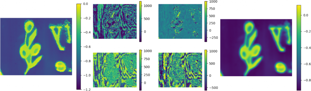
Measuring Confidence
While providing a confidence value of each pixel to the bilateral solver (introduced in the next section) is optional, we are currently exploring multiple heuristics to measure confidence of the initial phase estimate from EnvelopeNet. This will allow the denoiser to keep areas with high confidence while strongly denoising areas with low confidence.
- Observed Fisher Information: based on variance (over the four samples) of optimal phase value
- Fisher Information: based on expected variance of optimal phase values
- “Signal to Noise Ratio” between amplitude of interference term and non-interference term
- Parametrization of Observed Fisher Information as a MLP to learn optimal confidence
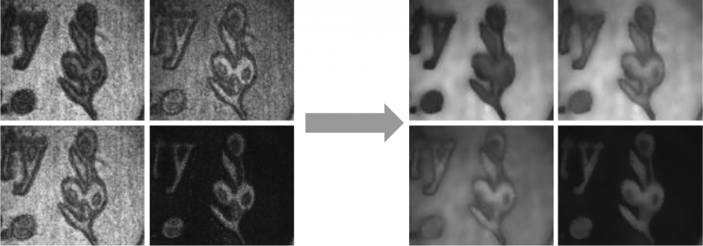
Differentiable Bilateral Solver
Since the loss used to train EnvelopeNet is between the output depth map and the ground-truth depth map generated by OCT, we need to be able to backpropagate through the complete pipeline, including the denoiser. This requires us to replace the bilateral filter, which is not differentiable, with the fast bilateral solver (Barron et al. 2015).
We get improved results even without optimizing the initial layers of our pipeline. The solver with an optimized value of λ parameter, which is a weight between the smoothness term and the fidelity term, already demonstrates results similar to ground truth in this example.