See Introduction for a description of the background and rationale behind these updates.
Poisson-Noise MLE
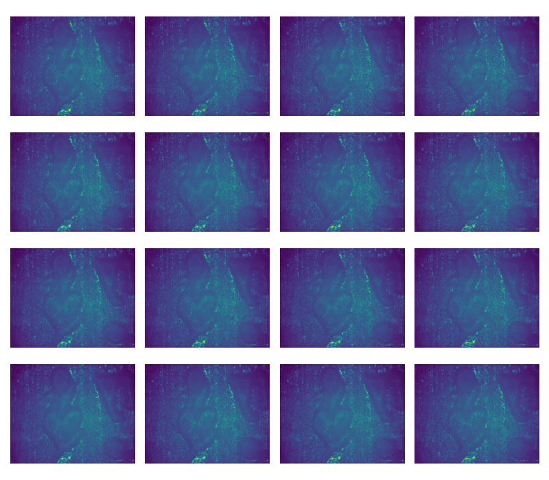
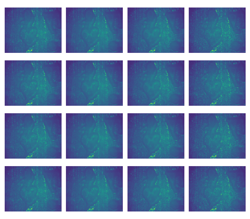
The classical phase-retrieval pipeline from Kotwal et al. 2022, as described in the Introduction, assumes a Gaussian noise model. While this is an appropriate model for read (sensor) noise, which is related to a camera’s circuitry and sensitivity, we can expect noise in the SWI frame capture process to be dominated by shot noise, which follows a Poisson distribution.
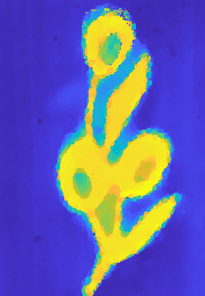
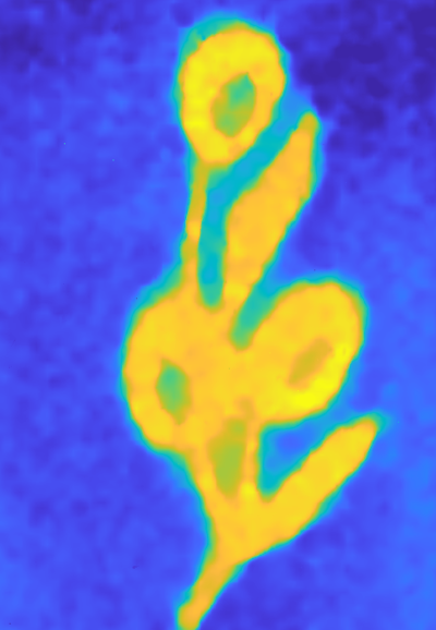
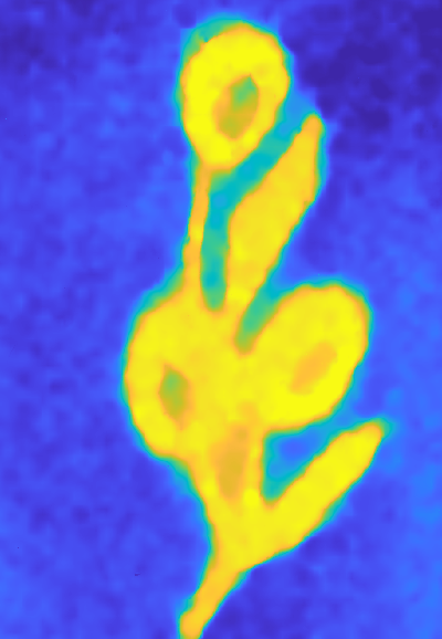
Changing the classical reconstruction pipeline to implement an MLE based on a Poisson noise model improves the output reconstruction by some 10%. Note the clearer boundaries and flatter surfaces in the Poisson reconstruction on the right.
Self-Supervised Image Formation MLP
Eventually, our goal is to demonstrate a neural network that incorporates the results of this project into a learned phase-recovery function that performs better than the classical pipeline. We know that this network will contain the differentiable bilateral solver as a module, but the rest of the architecture is still being designed.
A simple approach is to implement phase retrieval as a pixelwise MLP. This MLP should be able to learn different representations of the underlying data. One particularly useful representation to learn is a four-parameter image formation model, which can then be used to reconstruct the sixteen intensity images we started with.
This is a useful representation for two reasons:
- The fact that we can fully reconstruct the intensity images means that we can train the network in a self-supervised fashion. Since the intensity images are the input and the image formation parameters are the output, the reconstructed intensity images lend themselves to a natural reconstruction loss function with no need for ground-truth labels.
- One of the output image formation parameters is the phase, which is more or less the goal of the pipeline (since the phase difference is proportional to depth).
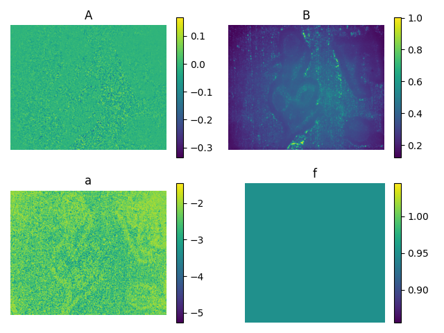
In particular, the four image formation parameters, denoted A, B, a, and f, satisfy the following relationship to the intensity I for each of i ∈ {0, 1, 2, 3} and j ∈ {0, 1, 2, 3} (that is, the grid of M times N shifts according to the method used to capture the intensity images):

Note that in this model, A, B, a, and of course I vary according to pixel location u,v, while f does not. Accordingly, the neural network is trained to learn an explicit parameter f and output A, B, and a.
Confidence measure using error propagation
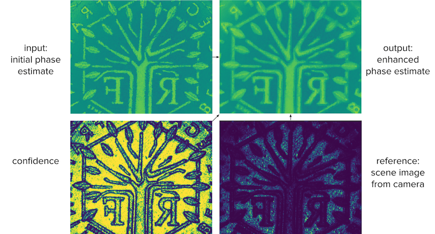
We represent the confidence of our initial phase estimate using error propagation on the first-order Taylor approximation of f, the phase estimation function (in our case MLE). First we take the Taylor approximation:

using the formula for error propagation (or variance propagation), we retrieve the estimated variance of the output of our estimation function:


We take the inverse of the variance as our confidence metric by calculating a using autodiff libraries:

This method can be generalized to any neural network by setting f as the network, as long as we can use autodiff to approximate the first-order derivative of the output with regards to the input. Providing the confidence image as input to the Fast Bilateral Solver resulted in a 70% error reduction in the final depth estimation compared to using the Fast Bilateral Solver with a constant confidence value, which would be equivalent to applying a bilateral filter.