Method
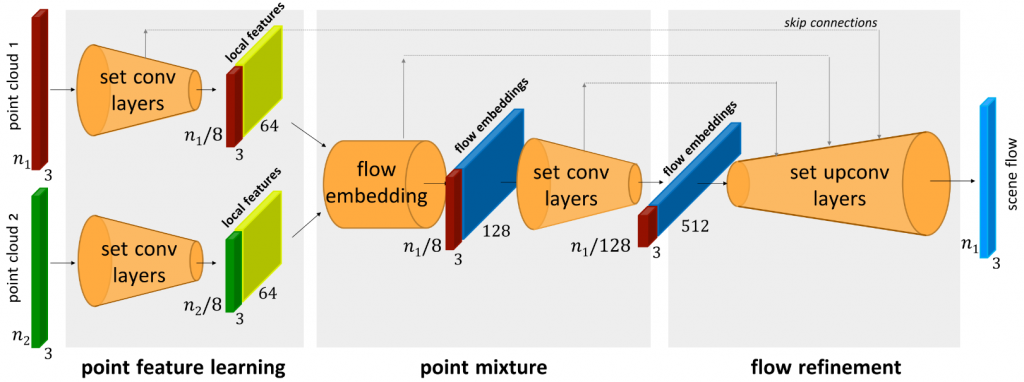
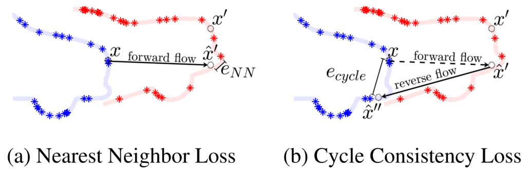
In this section, we will introduce the method we built for self-supervised scene flow estimation for deformable objects in detail. Our method is based upon the work Just Go With the Flow [1]. It is an extension from FlowNet3D [2] from supervised leanring to self-supervised learning, as shown in Figure 1. Just Go With the Flow focuses on scene flow estimation in rigid body scenarios, such as self-driving cars. We started from this baseline and modified it to work on non-rigid objects in our case.
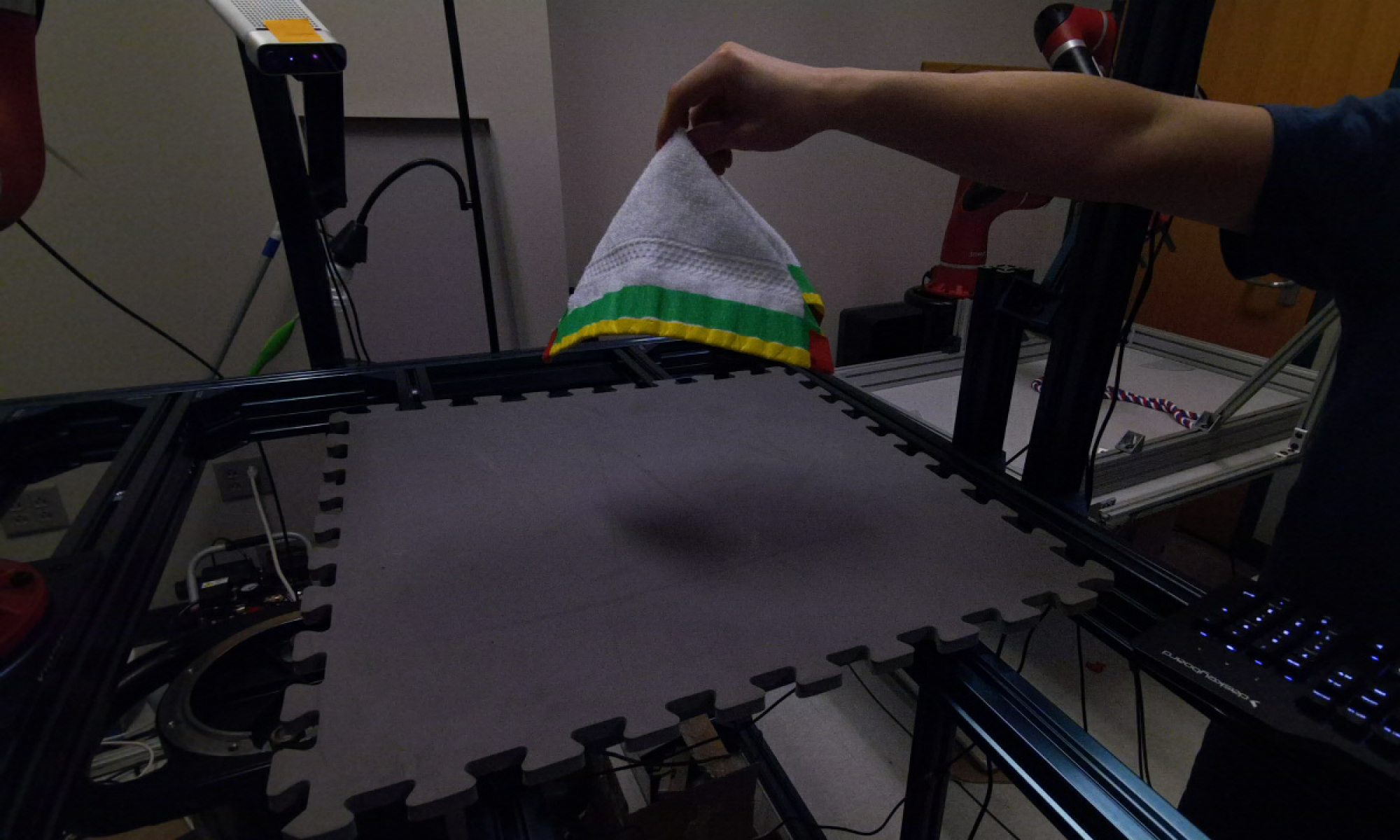
One major issue when we applied Just Go With the Flow to deformable objects is the vanishing training signal. We observed that when we use consecutive frames of point cloud to train the network, the learned flow prediction collapsed to zero vector. Our analysis on this phenomenon is that deformation between consecutive point clouds in our dataset is too small to supervise a meaningful flow prediction, so that the flow prediction degenerates to the trivial solution. We then experimented with different frame intervals between the pair of point clouds used in training, as shown in Figure 2.

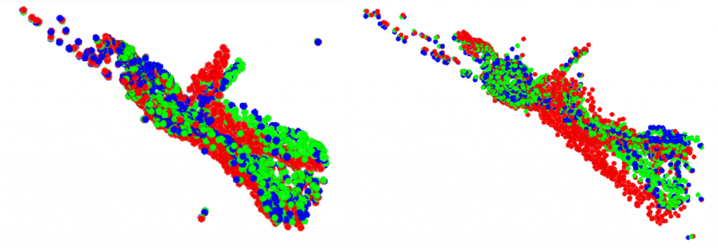
Now we will show some flow estimation results with different frame intervals used in training. In Figure 3, we show the flow prediction result when frame interval equals to 1. We can observe that the relative magnitude of the predicted flow is not large enough to move the original point cloud closely to the target point cloud.
Results
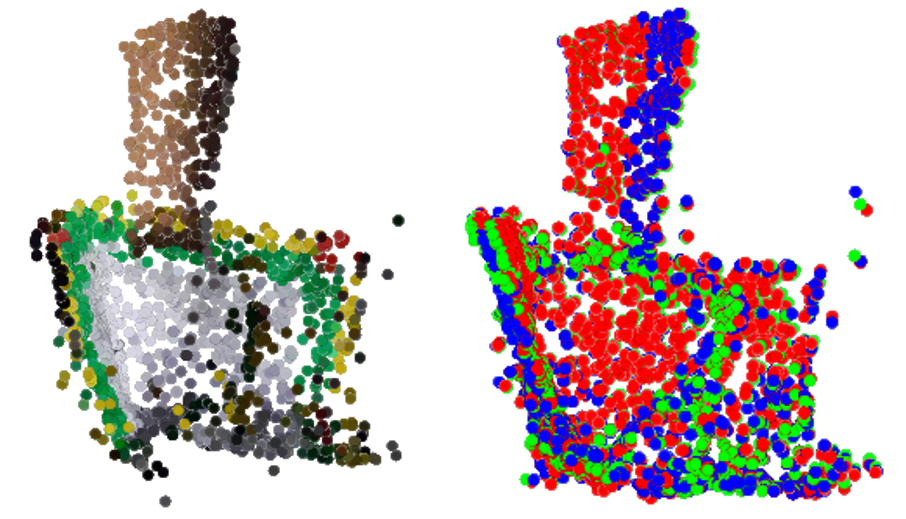
Red: Original point cloud
Blue: Pseudo-GT
Green: Prediction (original point cloud + estimated flow)
In Figure 4 and Figure 5, we further increased the frame interval to visualize the predicted flow. We can observe that the predicted point cloud can still align well with the original point cloud even under large frame intervals.
Red: Original point cloud
Blue: Pseudo-GT
Green: Prediction (original point cloud + estimated flow)
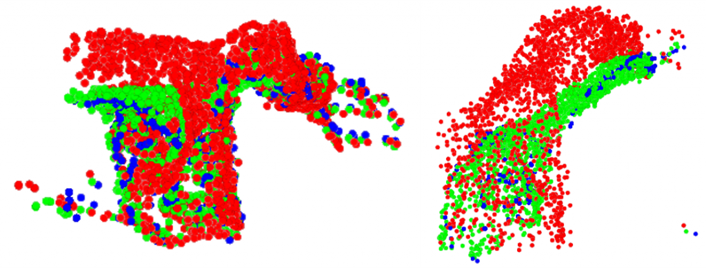
Red: Original point cloud
Blue: Pseudo-GT
Green: Prediction (original point cloud + estimated flow)
We chose to use frame interval = 5 at last because it doesn’t degenerate the predicted flow to trivial solution or make the flow prediction too ambiguous under large deformation.
References
[1] Mittal, Himangi et al. “Just Go with the Flow: Self-Supervised Scene Flow Estimation.” ArXiv abs/1912.00497 (2019): n. pag.
[2] Liu, Xingyu et al. “FlowNet3D: Learning Scene Flow in 3D Point Clouds.” 2019 IEEE/CVF Conference on Computer Vision and Pattern Recognition (CVPR) (2019): 529-537.