Self-supervised Embedding Prediction - Self-supervised Representation Learning for Deformable Objects

Method

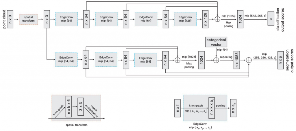
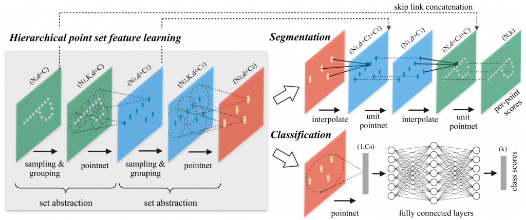
In this section, we will introduce the method we built for self-supervised embedding prediction for deformable objects in detail. Our method makes use of an encoder-decoder network to predict an embedding for every point in the point cloud. Here we used Dynamic Graph CNN [1] and PointNet++ [2] as our backbone to do experiments, as shown in the figure below.

Network Architecture of Dynamic Graph CNN. We used the segmentation branch of the network.

*Network Architecture of PointNet++. We used the segmentation branch of the network.*

The losses we used to train the embedding prediction network are the followings:

Triplet loss (margin = 1)
L2 norm loss: To enforce the L2 norm of the embedding to be 1.
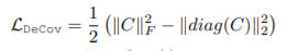
Covariance loss: To minimize correlation between different embedding channels.

Covariance loss function proposed in [4].

Results

We show the histograms of embedding values at different channels and different epochs in the figure below.

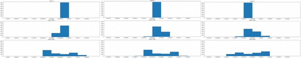
Visualization of the embedding value distribution.
Horizontal axis: channel 1 – 3
Vertical axis: epoch 1 – 3

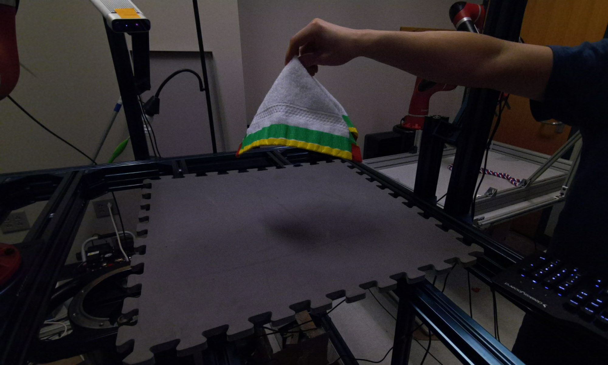
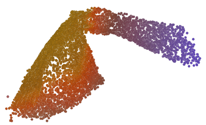
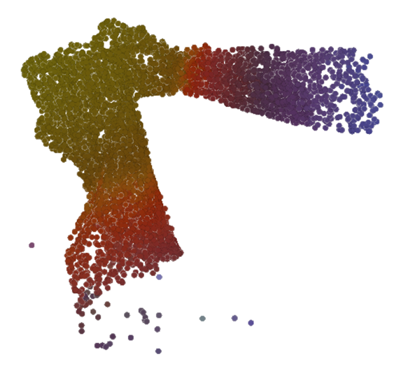
We show some colored visualizations of the predicted embedding values in the figures below. Here we set the size of the predicted embedding vector to be 3. Then we normalized the values of each embedding channel to be in the range [0, 1]. Lastly we colored the RGB channel of each point using the 3-dimensional embedding vector. This visualization method maps the embedding distance to color affinity. The closer the two colors are, the closer the two points are in the embedding space.

Here we observed that the embedding prediction results are not good enough yet. Ideally we would want the model to fully learn semantic meaning of the point cloud. But the model is not able to distinguish between the towel and the hand yet. It only has the sense of the “center” of the whole object, including the towel and the hand, and the relative distance from the center to edges. For now the articulation point of the hand and the towel is treated as the “center”. This should largely due to the bias in the training dataset, where the arm and the towel appear to be linked by the “center”. Consequently, the model regarded the wrist and the lower edge of the towel as similar points. We imagine semantic segmentation labels may be helpful for learning better embedding values.

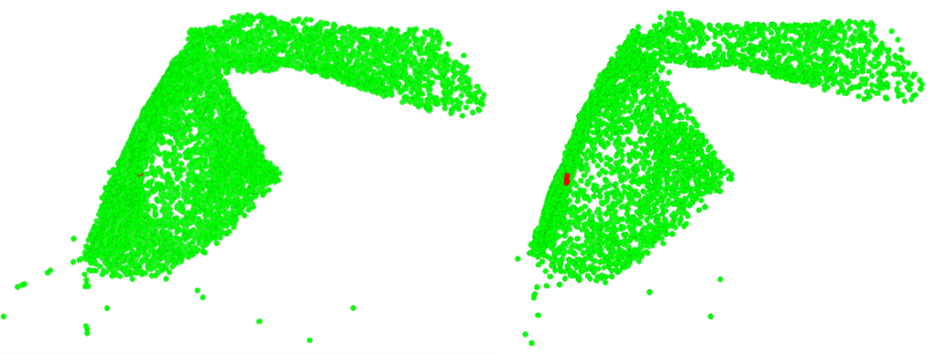
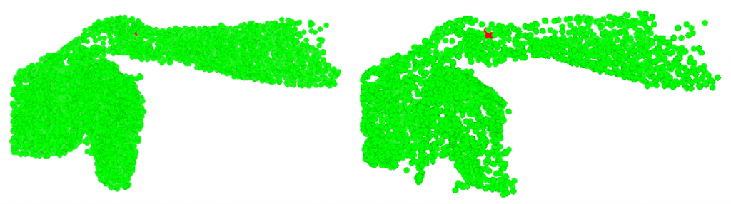
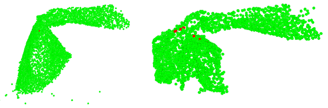
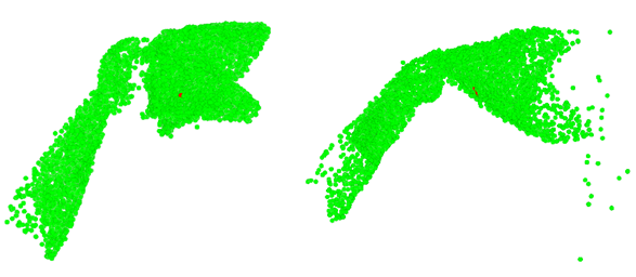
We show the predicted correspondences indicated by the nearest neighbors in the embedding space in the figures below. Red point in the left figure is the sampled point. Red points in the right figure are the nearest neighbors to the sampled point in embedding space.

When frame interval is small:

Frame 300 (left) and 305 (right). The correspondences are predicted correctly at the center of the towel.

*Frame 500 (left) and 505 (right).* *The correspondences are predicted correctly on the wrist.*

*Frame 700 (left) and 705 (right). The correspondences are predicted roughly correctly near the edge of the towel.*

When frame interval is large:

*Frame 300 (left) and 500 (right). The correspondences are predicted roughly correctly at one corner of the towel near the hand.*

*Frame 500 (left) and 700 (right). The correspondences are predicted correctly at the center of the towel.*

We also made a visualization tool to show the correspondence prediction in real-time. The left window shows the point cloud 1 and the right window shows the point cloud 2. The point clouds are colored using 3 channels of embedding values. When the cursor is moving in the left window, the right window will show in real-time the true and predicted correspondence. Some screenshots of both success and failure cases are shown in the figures below.

Success cases:

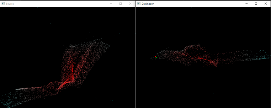
*Red dot: True correspondence indicated by the predicted flow*.
*Green dot: Predicted correspondence indicated by the embedding values*.

Failure cases:

References

[1] Wang, Yue et al. “Dynamic Graph CNN for Learning on Point Clouds.” ACM Trans. Graph. 38 (2018): 146:1-146:12.

[2] Qi, C. R. et al. “PointNet++: Deep Hierarchical Feature Learning on Point Sets in a Metric Space.” ArXiv abs/1706.02413 (2017): n. pag.

[3] Cogswell, Michael et al. “Reducing Overfitting in Deep Networks by Decorrelating Representations.” CoRR abs/1511.06068 (2016): n. pag.