Solution Framework
Given a text prompt as input describing the scene, we can divide the solution into the following parts:
- Text-to-Image Generation
- Artistic-to-Natural Image Translation
- Mask Generation
- Optical Flow Prediction
- Looping Video Generation
Text-to-Image Generation
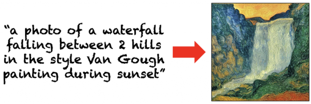
Using a pretrained Stable Diffusion model (in our case we use stable-diffusion-v1-4) we generate a single image corresponding to the text prompt. We use DDIM sampling (with 1000 steps) and classifier-free guidance (with a scale of 7.5).
Artistic-to-Natural Image Translation
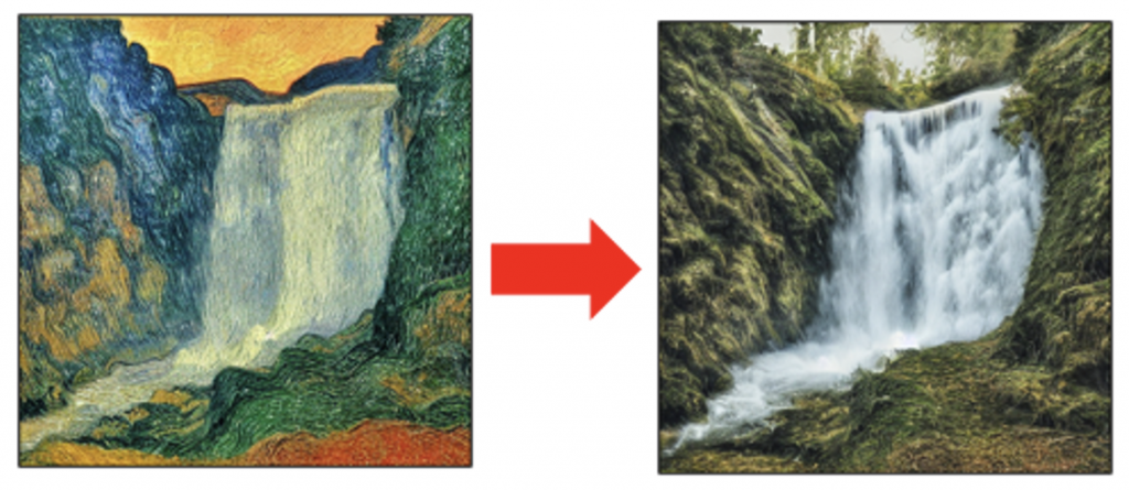
Since there are repeating textures in the image that we want to animate (like water in the waterfall region) we want to model the looping video generated by optical flow warping. We need to predict the optical flow from the single generated image. We have a dataset of real in-the-wild videos (that are natural videos), and thus, can not predict the optical flow for the generated artistic style image as it is out of the distribution of the training data.
Can we generate a natural version of this image? Since we generate images from Stable Diffusion, we have access to all the internal features (ResNetBlock outputs, Self-Attention Maps, and Cross-Attention Maps) we use a method of image editing similar to Plug-and-Play, where we use the same random noise along with internal features of ResNetBlock4 and Self-Attention Maps (after timestep 541) and the caption “waterfall, nature, jungle, bright, realistic, photography, 4k, 8k” to generate the natural version of the artistic image, having the same semantics.
Mask Generation
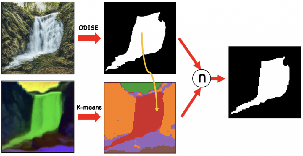
The optical flow prediction model also requires a mask, which defines which regions to move. We experimentally verified that this is extremely crucial to the prediction of a reasonable optical flow for animation and ensuring that regions that should otherwise be stagnant (like rocks and mountains) should not move.
We use a pretrained ODISE image segmentation model to segment the edited natural image. However, we do not use this mask directly as there might be some inconsistencies at boundaries between the artistic image and its edited natural counterpart. We perform a KMeans clustering of the Self-Attention maps, which gives us a nice clustering and then we identify which regions in the cluster correspond to those in the ODISE segmentation map and choose those to be part of the mask. Finally, to refine the mask, we take an intersection of the ODISE mask and the one obtained from Self-Attention Maps.
Optical Flow Prediction
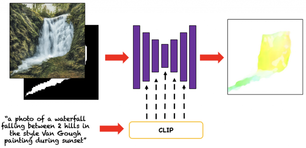
Given the edited image, mask, and the text-prompt we predict a single optical flow that can describe the motion between each pair of consecutive frames in the generated video. We use Cross-Attention conditioning (similar to Stable Diffusion) to use text conditioning. Since the dataset of real videos does not contain text descriptions, we use text prompts generated by BLIP2 (from a single video frame).
Looping Video Generation
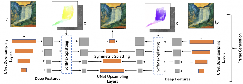
Since the semantic layout of the edited natural image is similar to the artistic image, we can use the optical flow predicted for the edited natural image to animate the artistic image. Taking the same artistic frame as the start and end frame of the video, we predict a given frame at time t by first Euler-integrating the optical flow in the forward direction (0->t) and backward direction (N->t-N) and then do symmetric splatting in the feature space rather than RGB space, followed by a decoder to predict the t-th RGB frame.
To better understand the euler-integration we explain it using the equations below:
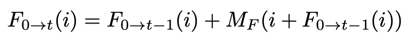
Using the optical flow prediction network, we predict M_F which denotes the optical flow between any 2 consecutive frames in the video, (i.e., M_F = F(0->1), or F(1->2)). In order to get the flow from 0 to the t-th frame, we get F(0->t) using the recursive integration formula shown above.
References
- Holynski, Aleksander, et al. “Animating pictures with eulerian motion fields.” Proceedings of the IEEE/CVF Conference on Computer Vision and Pattern Recognition. 2021.
- Mahapatra, Aniruddha, and Kuldeep Kulkarni. “Controllable Animation of Fluid Elements in Still Images.” Proceedings of the IEEE/CVF Conference on Computer Vision and Pattern Recognition. 2022.
- Tumanyan, Narek, et al. “Plug-and-Play Diffusion Features for Text-Driven Image-to-Image Translation.” arXiv preprint arXiv:2211.12572 (2022).
- Xu, Jiarui, et al. “Open-vocabulary panoptic segmentation with text-to-image diffusion models.” arXiv preprint arXiv:2303.04803 (2023).