Approach

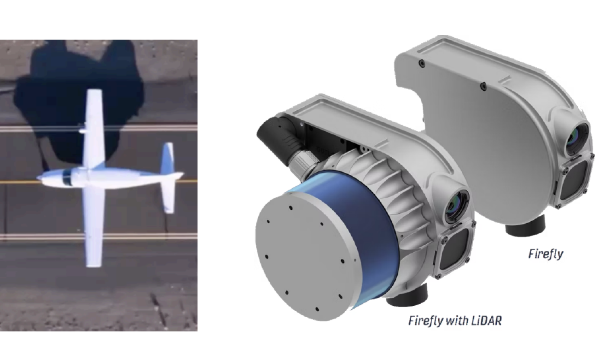
We first evaluate current SOTA zero-shot metric and relative depth models directly on NEA’s data suite, quantifying where and how these failure modes manifest in the Firefly’s specific operational environment. This evaluation drives our approach down one of two paths:

Path 1 — No Existing Model Generalizes Sufficiently

We deploy a learning-based framework that treats sparse LiDAR points as geometric anchors. We can fuse through the following steps:

Step 1- LiDAR Projection into Image Plane

$$\begin{bmatrix} u_i \\ v_i \\ d_i \end{bmatrix} = \mathbf{K} [\mathbf{R} | \mathbf{t}] \begin{bmatrix} X_i \\ Y_i \\ Z_i \\ 1 \end{bmatrix}, \quad (u_i, v_i) = \left(\frac{u_i}{d_i}, \frac{v_i}{d_i}\right)$$

Step 2 – Anchor Correspondence

$$\mathcal{A} = \{(d^r_i,\ d^L_i)\} \quad \text{where} \quad d^r_i = D^r(u_i, v_i)$$

Step 3 – Affine Calibration via Least Squares

$$\min_{s,\, t} \sum_{i} \left( s \cdot d^r_i + t – d^L_i \right)^2 \quad \Rightarrow \quad [s,\ t]^\top = (\mathbf{A}^\top \mathbf{A})^{-1} \mathbf{A}^\top \mathbf{b}$$

Step 4 – Dense Calibrated Depth Map

$$D_{\text{cal}}(u, v) = s \cdot D^r(u, v) + t$$

Step 5 – Total Fusion

$$D_{\text{fused}}(u, v) = \begin{cases} d^L_i & \text{if } (u, v) \in \mathcal{A} \\ D_{\text{cal}}(u, v) & \text{otherwise} \end{cases}$$

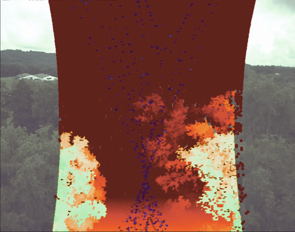
Example showcasing a partial image showcasing LiDAR data overlaid the RBG frame.

Ransac Optimization

While total fusion recovers a dense metric map, the global least squares solve in Step 3 can become a bottleneck at runtime. RANSAC offers a robust, faster alternative by operating over a sampled subset of anchors.

One particular way we can improve runtime efficiency, is by solving a least squares optimization and fitting an affine model via RANSAC, such that at each iteration, we sample k-anchor pairs per iteration to find the best scale s and shift t values. Using anchor set A from Steps 1–2:

Step 3 – Affine Model per RANSAC Iteration

$$d^L = s \cdot d^r + t \quad \Rightarrow \quad [s,\ t]^\top = \mathbf{A}_k^{-1}\, \mathbf{b}_k$$

where $\mathbf{A}_k$​ and $\mathbf{b}_k$​ are constructed from $k$ sampled anchor pairs per iteration.

Step 4 – Inlier Scoring

$$\mathcal{I}^* = \arg\max_{s,\,t} \left|\left\{ i \in \mathcal{A} : \left| s \cdot d^r_i + t – d^L_i \right| < \epsilon \right\}\right|$$

Step 5 – Calibrated Depth Map

$$D_{\text{cal}}(u, v) = s^* \cdot D^r(u, v) + t^*$$

This yields a calibrated depth map recovering accurate absolute metric depth across the full scene without the payload and cost overhead of a dense LiDAR system.

Potential Further Optimization

We can also go with a structure-aware approach over the image, where we first determine interest points (places where depth changes greatly), and sample any points from said regions. From there, can we pass k-anchor pairs to our RANSAC algorithm. This may have the RANSAC algorithm converge faster, at a cost of prior sampling of interest points.

Path 2 — Candidate Model Exists

If a strong candidate model¹ exists, then we can natively run the model as is. However, it is very likely (and confirmed through our tests) that the model suffers from a domain shift. To rectify, we fine-tune it directly on NEA’s data suite. This path explores whether domain adaptation alone can close the performance gap — potentially eliminating the need for LiDAR at runtime time altogether.

Both paths are evaluated against the same NEA ground truth benchmark. The benchmark is provided by a posterior scene reconstruction, from LiDAR data. This enables a principled, data-driven decision about which approach best balances accuracy, hardware constraints, and deployment feasibility for the Firefly system. The cons of this approach would be potential lack of fine-grained details, as well as a potential need for modeling trees (the unstructured objects that dominate the scenery).

---

Footnotes

1. A strong candidate model is defined as one with strong metric depth estimation relative to the LiDAR ground truth, or a model with structurally sound relative depth estimation (in other words, we allow for scale ambiguity). Ideally, the candidate model runs inference without utilizing too much GPU memory, and is computationally fast enough to avoid hindering downstream tasks. ↩︎