In this section, we validate our method (ITI-Gen) for inclusive text-to-image generation on various attributes and scenarios.
Single Binary & Multiple Attributes
To demonstrate the capability of our method to sample images with a variety of face attributes, we construct 40 distinct reference image sets based on attributes from CelebA [1]. Also, given multiple reference image sets (each captures the marginal distribution for an attribute), ITI-GEN can generate diverse images across any category combination of the attributes.
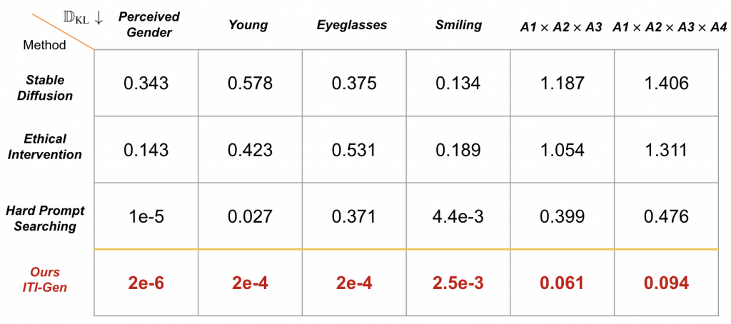
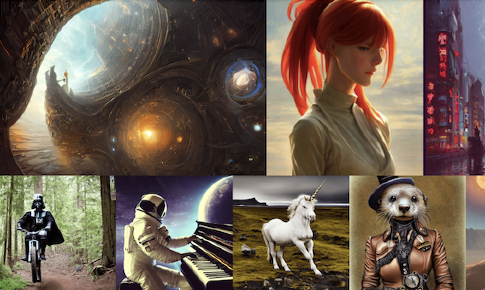
We evaluate 5 text prompts in Figure 1— “a headshot of a {person, professor, doctor, worker, firefighter}” — and sample 200 images per prompt for each attribute, resulting in 40K generated images. We highlight the averaged results across 5 prompts of 6 attributes. ITI-GEN achieves near-perfect performance on balancing each binary attribute and multiple attributes, justifying our motivation: using separate inclusive tokens is beneficial in generating images that are uniformly distributed across attribute categories.
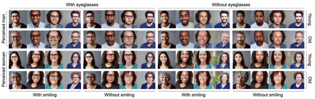
In Figure 2, we show the qualitative results of our method in debiasing 4 binary attributes simultaneously. The results show that our method perform well in debiasing multiple attributes.
Multi-Category Attributes
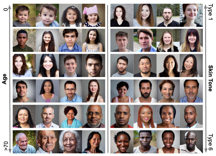
We further investigate multi-category attributes including perceived age and skin tone.
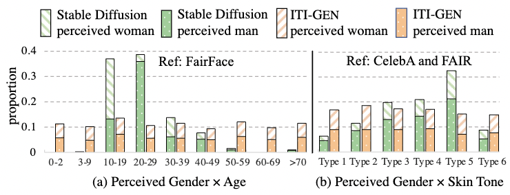
Specifically, we consider two challenging settings: (1) Perceived Gender × Age (Figure 4(a)), and (2) Perceived Gender × Skin Tone (Figure 4(b)). ITI-GEN achieves inclusiveness across all setups, especially on extremely under-represented categories for age (< 10 and > 50 years old in Figure 4(a)). More surprisingly (Figure 4(b)), ITI-GEN can leverage synthetic images (from FAIR) and jointly learn from different data sources (CelebA for gender and FAIR for skin tone), demonstrating great potential for bootstrapping inclusive data generation with graphics engines.
Other Domain
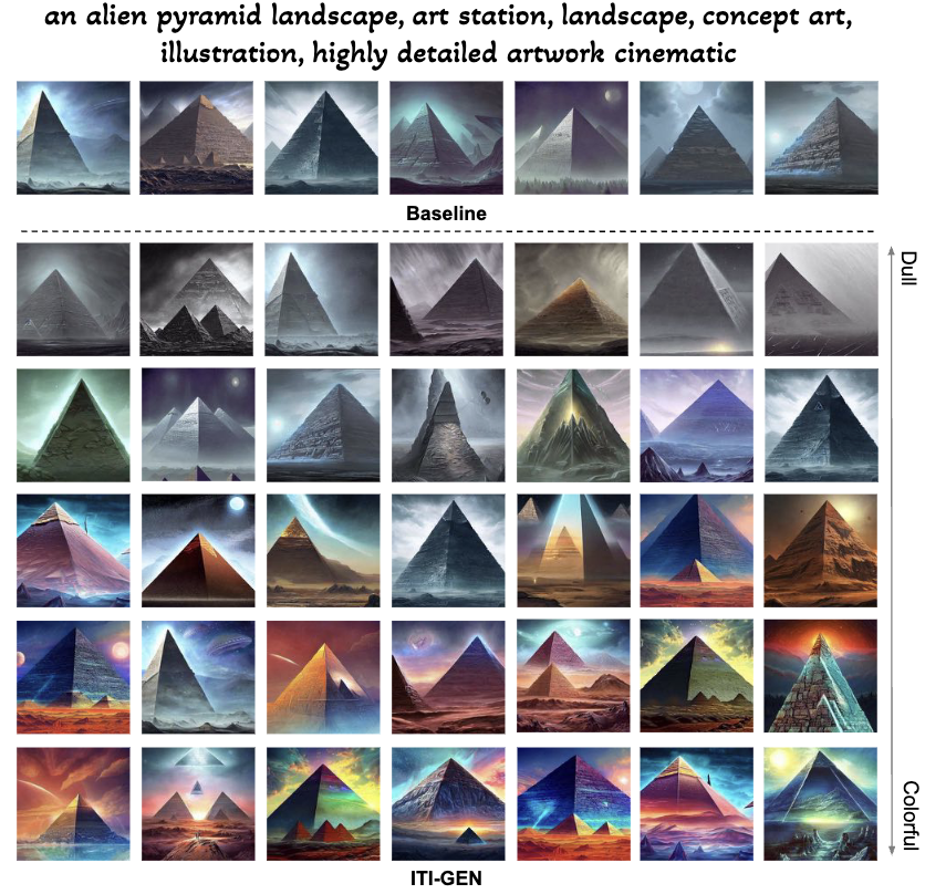
Figure 5. ITI-GEN with perception attributes (“Colorfulness”) on scene images. The tokens of “colorfulness” are trained with “a photo of a natural scene” and applied to “an alien pyramid landscape… ” in this example. ITI-GEN (bottom) enables the baseline Stable Diffusion (top) to generate images with different levels of colorfulness.
Besides human faces, we apply ITI-GEN to another domain: scene images. We claim that the inclusive text-to-image generation accounts for attributes from not only humans but also scenes, objects, or even environmental factors. Specifically, we use images from LHQ [2] as guidance to learn inclusive tokens and generate images with diverse subjective perception attributes. As illustrated in Figure 5, ITI-GEN can enrich the generated images to multiple levels of colorfulness, justifying the generalizability of our method to the attributes in different domains.
In conclusion, the results above demonstrate the effectiveness of our method in debiasing different attributes and different scenarios.
References:
[1]. Ziwei Liu et al. “Deep learning face attributes in the wild.” In ICCV, 2015
[2]. Ivan Skorokhodov, et al. “Aligning latent and image spaces to connect the unconnectable.” In ICCV, 2021.