Baseline
For our baseline, we plan on using the ‘End-to-End Learning for Omnidirectional Stereo Matching With Uncertainty Prior[1] paper. The original setup involves a four fisheye camera setup. We implemented this from scratch for our camera setup and data
Summary
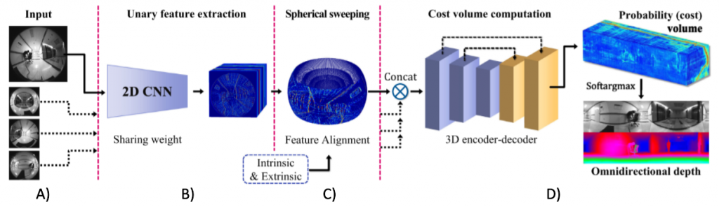
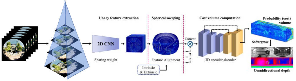
- Sphere Sweep (C) – Every pixel of the six fisheye images is projected onto n spheres. These spheres lie evenly between the minimum and maximum depth to be measured.
- For every pair of images, the n spherical representations are integrated and then averaged over to form a 4D cost volume.
- The cost volume is then passed through a 3D encoder-decoder to generate the depth map (D).
- To save on computation and memory, sphere sweep is run on feature maps generated by a 2D CNN feature extractor (B) instead of the images themselves.
Uncertainty Prior
In case of hard matching cases such as textureless, reflective, or occluded regions, the depths predicted might not be accurate enough. In such cases, having a confidence measure of the model predictions would provide a good indication of where the model doesn’t perform well. This measure would provide the model a great training signal to penalize such scenarios and detections appropriately.
One of the novel ideas presented in this paper included having an uncertainty prior. The uncertainty, measured using entropy, information would be used to filter out depths with uncertainty higher than a threshold. This information would also be used to enforce an uncertainty loss thus, forcing the model to learn such cases explicitly.
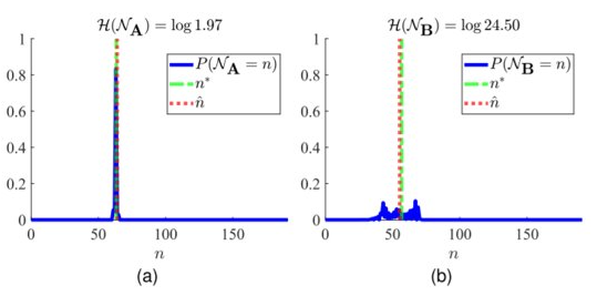
The graphs above two scenarios of depth prediction. In (a), the depth is predicted with high probability. The predicted depth is close to the ground truth depth and so, the overall loss is low and the uncertainty loss is low as well. In (b), however, the depth predicted is very close to other depth candidates around it. Fortunately, the predicted depth turned out to be very close to the ground truth depth. So, the loss is low. However, due to the low and distributed probabilities, the entropy is high and the overall uncertainty loss is high. The model is thus, forced to disambiguate such scenarios.
This uncertainty prior is yet to be implemented.
Analysis
Double Sphere Camera Model
Due to the extreme distortion that a fisheye lens produces, the pinhole camera model doesn’t apply. There are several models such as the Fisheye Projection Model[1] and the Kannala-Brandt Camera Model[2] which could be used. However, the inverse projection (3D point to 2D) either requires solving an optimization problem or expensive trigonometric operations. Enter Double Sphere Camera Model[3].
In order to verify that this model worked and to test that the project and inverse projection matched, we performed a small test. By taking a mask similar to a fisheye image, we projected each pixel to 3D space and then reprojected these back to the image plane. Both these operations were performed using the formulae defined by the Double Sphere Camera Model. The resulting pixel locations were compared with the original pixel locations and the projection errors were plotted.
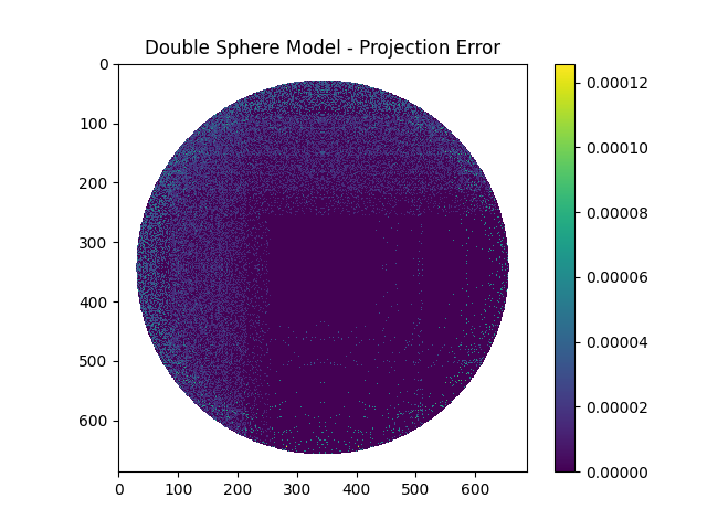
As can be observed, the maximum error was below a pixel separation of 0.0001 which was definitely acceptable. Thus, this camera model would work well for our project.
Determining Output Size
As part of our pipeline, the six fisheye images are stitched together into a panorama image.
The input fisheye size is fixed due to the compute constraints and the requirements of the other modules. However, the output panorama resolution needs to be determined.
- It can’t be too low or else we wouldn’t be able to leverage the information captured by the input images.
- It can’t be too high or else there is a possibility that an input image pixel might correspond to more than 1 output pixel. This could lead to incorrect/blurry depth estimation.
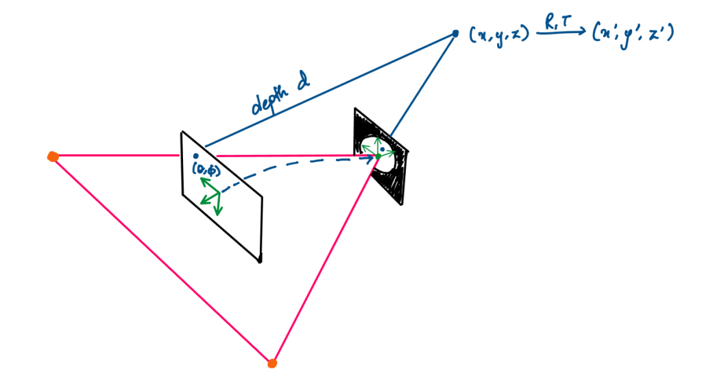
To calculate this correspondence
- An output pixel (denoted by
(theta, phi)) is projected to the 3D space in the Panorama frame –(x, y, z). - It is then moved to the 3D space in a particular Camera’s frame –
(x', y', z'). - Using the Double Sphere model, it is inversely projected onto the fisheye image plane.
- This is done for each output pixel and the difference with its neighbors is calculated.
Using the above methodology, we conducted our analysis.
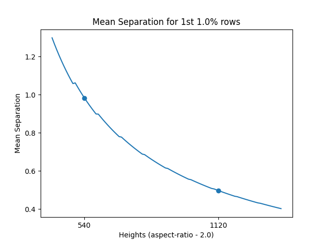
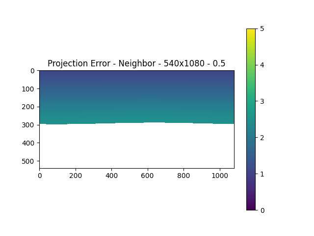
For an input size of 1224x1028, we found that at a height of 540px (and a width of 1080px – maintaining an aspect ratio of 2), the mean separation error for the 1st 1% rows just goes below 1px. Therefore, for any heights less than or equal to 540px, the minimum pixel separation would be above 1. This can be seen in the actual projection error heatmap as well.
The reason why we consider the top rows is because that’s the area, in a panorama image, that constitutes maximum distortion. Unlike the part of panorama images that represent forward, left, or right, the top view is covered by the entire width and so, the limited input pixels corresponding to the top view need to make up for the entire top rows. This would lead to maximum duplication of information.
Alternative Approach
SliceNet
An alternative approach to solving MVS using Sphere Sweep and Cost Volume Computation, would be to predict depth using a single panorama image view. Intuitively, this makes sense as in all cases, the model outputs a panorama depth map anyway.
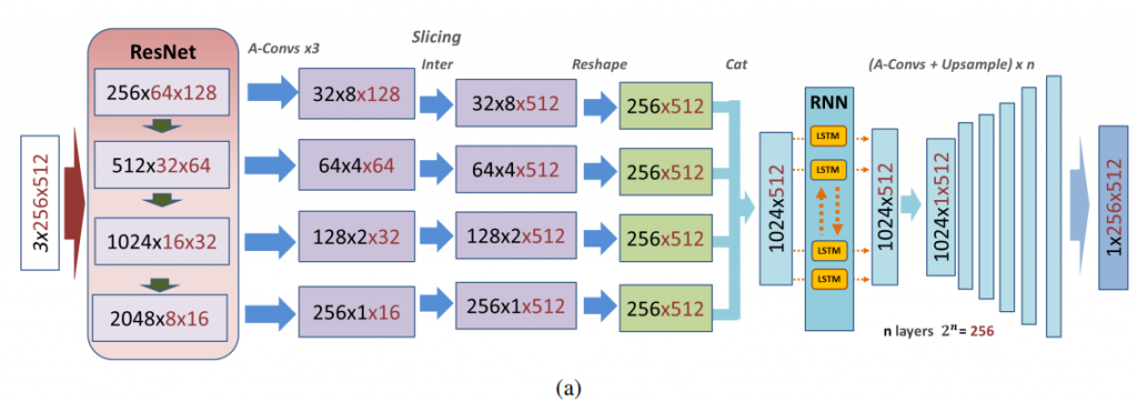
SliceNet[1] estimates depth from a single input panorama image.
- Panorama image is fed to a pretrained ResNet50 feature extractor.
- The last 4 layer outputs are used to ensure that both, high level details and spatial context, are captured.
- These outputs are passed through 3 asymmetric 1×1 convolutional layers to reduce the channels and heights by a factor of 8.
- The width component is then resized to 512 by interpolation and the reshaped components are concatenated to get 512 column slices of feature vectors of length 1024.
- These slices sequentially represent the 3600 view and so, are passed through a bi-directional LSTM setup.
- The reshaped output is then upsampled to obtain the depth map.
The authors used an Adaptive Reverse Huber Loss[2] to train this network.
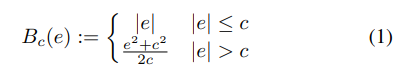
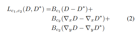
This loss is essentially a combination of L1 and L2 loss. However, just this alone wasn’t enough. As per studies[3], CNNs tend to lose details during tasks such as depth estimation. Thus, the training signal also included loss terms penalizing the gradient along X and Y. These gradients were calculated using horizontal and vertical sobel filters[4].
Dataset
Besides the above analysis and investigations, another problematic area seemed to be the dataset.
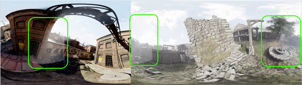
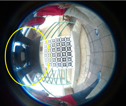
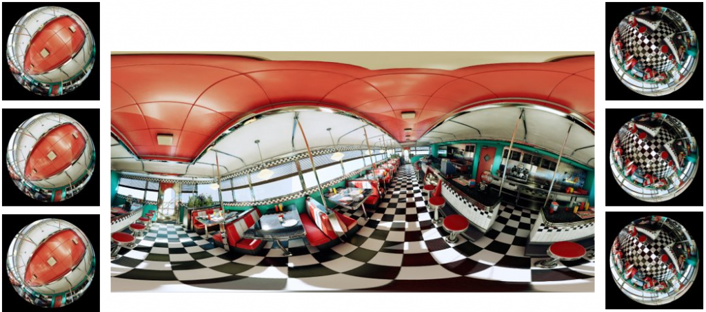
The above figure contains an example of the stitched panorama image from the old dataset. As can be seen in the green boxes, there are some weird lighting and fog related artifacts which seemed to be causing problems.
Besides these artifacts, another issue with the old dataset was the problem of redundant views. The way this synthetic dataset was generated led to a lot of redundancy in different images from the same scene/environment, and even similar viewing angles. Thus, we needed to start working on a new dataset.
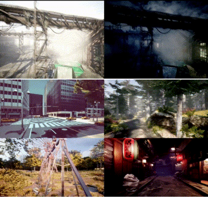
AirSim is a drone simulator built on Unreal engine by Microsoft Research. In the above figure, you can see the variety of environments – these range from urban to jungle landscapes, day to night, different weather conditions and lightings.
To generate this new dataset, we go through each environment and sample random points along the free area based on the occupancy graph. Through these points, random trajectories are generated. Along these trajectories, we randomly sample points and at such valid points, at random angles, we capture the required image.
Laplacian Model
We retrained baseline on the new dataset and we saw an improvement. However, there were still issues. And these seemed to be primarily due to the camera orientation restrictions
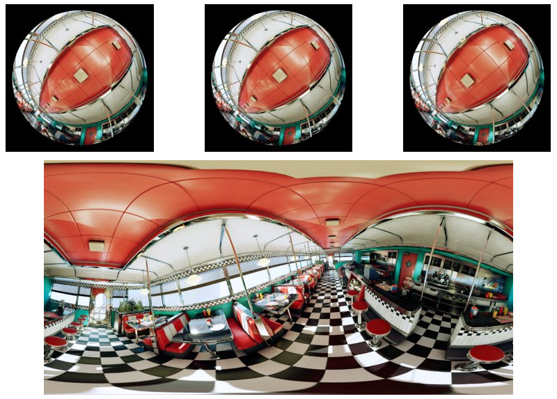
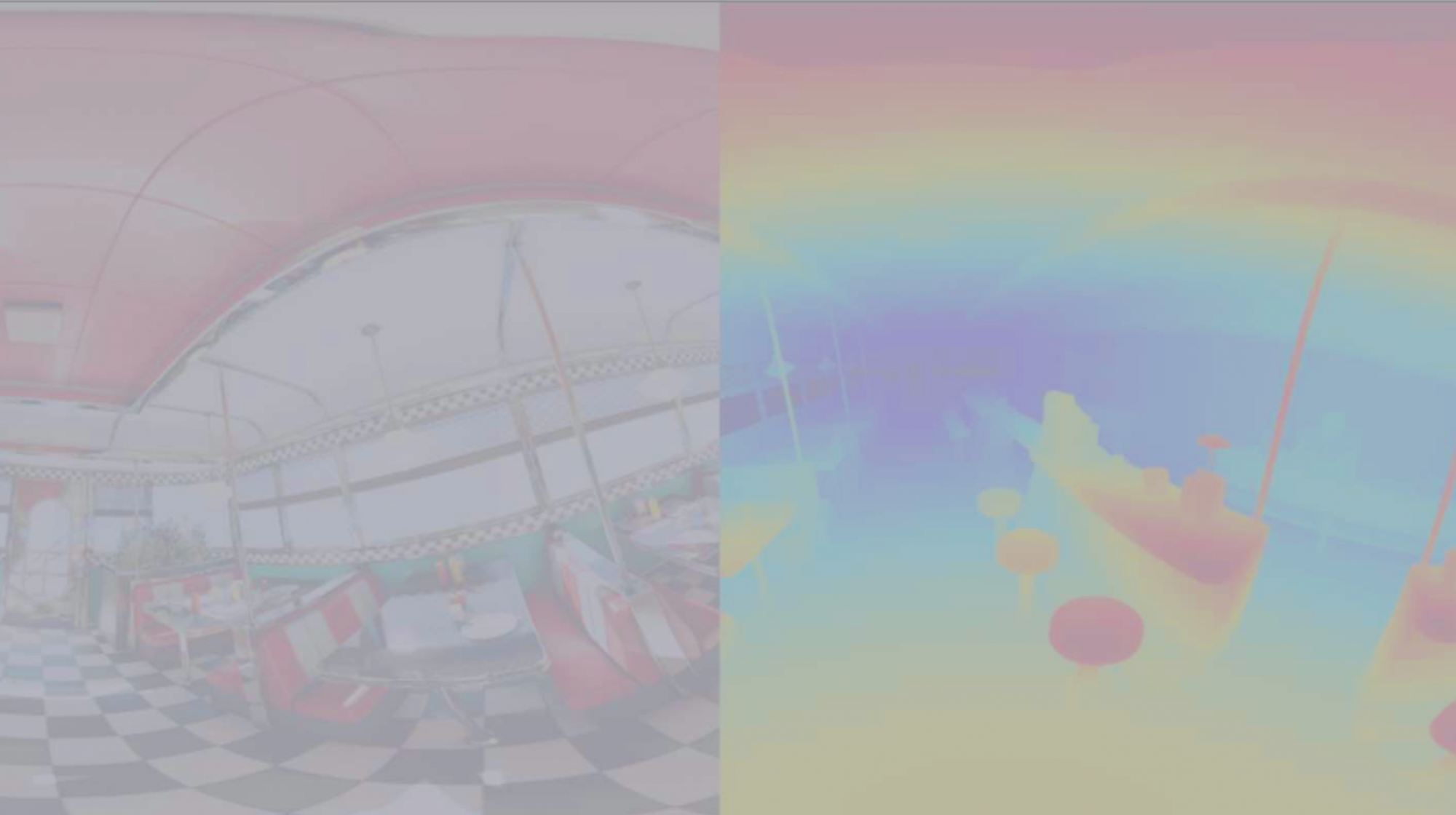
In the figure above, we can see the fisheye images corresponding to the top cameras and the ground truth panorama image. As can be seen, a majority of the undistorted portion of all the fisheye images highlight the same details of the scene. And a lot of the important environmental details are highly distorted.
Thus, to try and capture finer details, we modified the model to include a laplacian pyramid as shown below
The above showed improvements in capturing some of the finer details. This can be seen in the example below
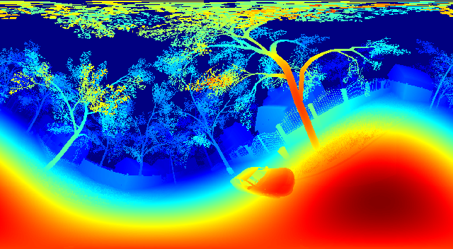
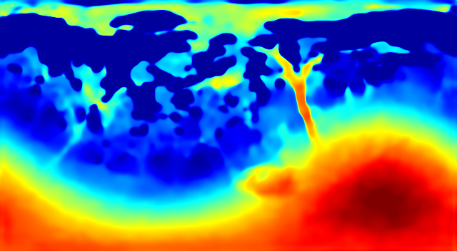
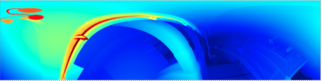
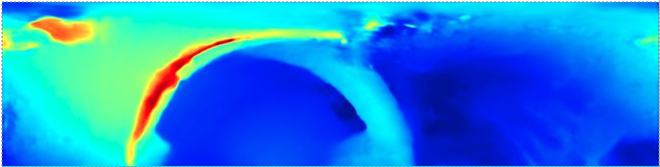
| Ground Truth | Prediction |
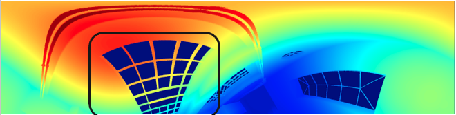 | 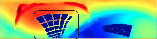 |
Results
Baseline Results
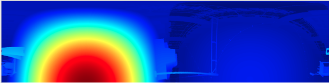
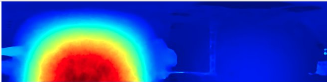
| Ground Truth | Prediction |
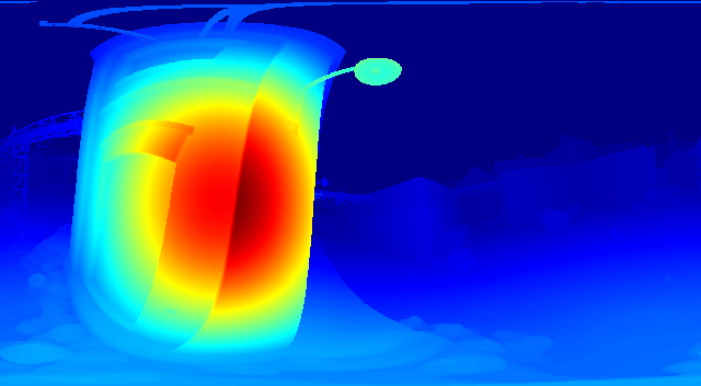 | 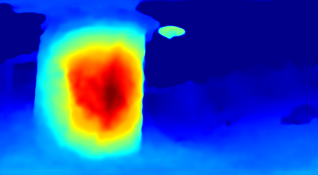 |
 |  |
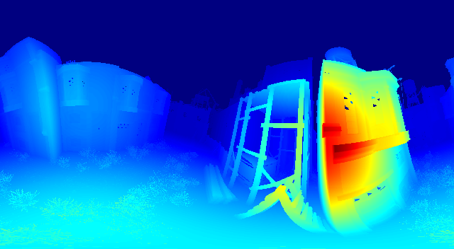 | 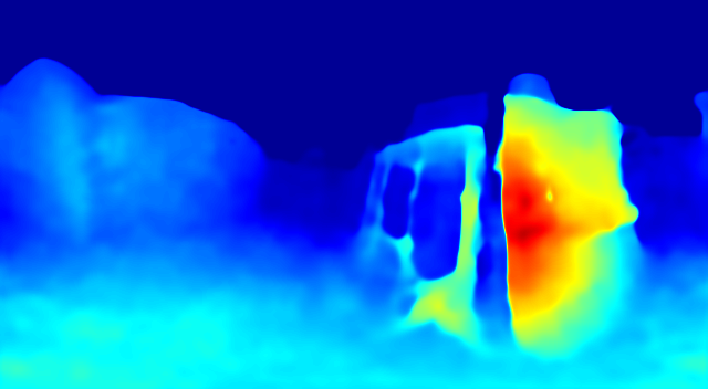 |
 |  |
 |  |
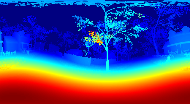
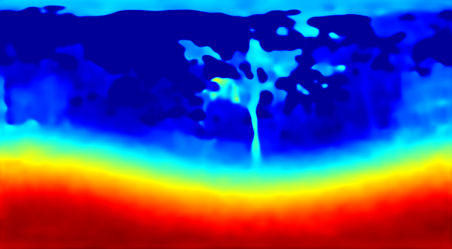
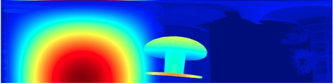
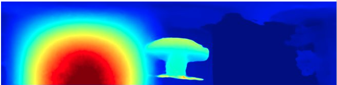
Laplacian Pyramid Model
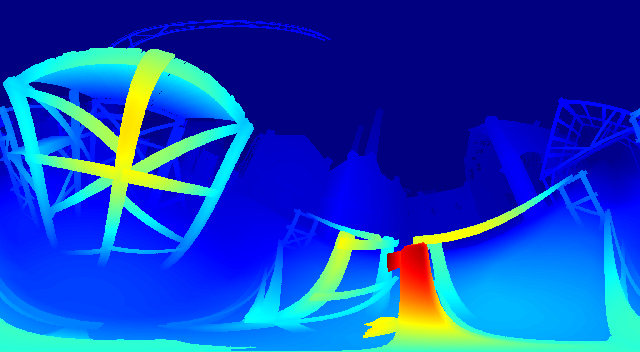
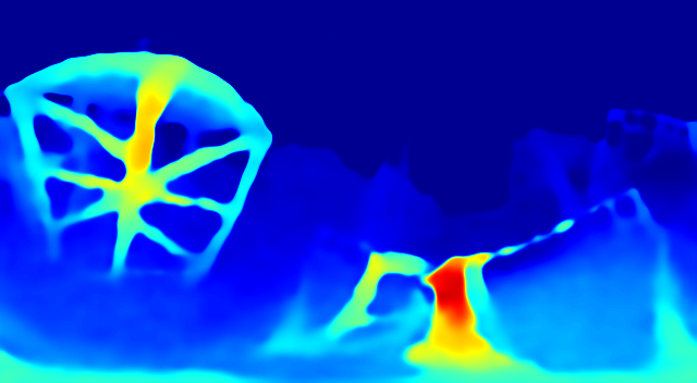
| Ground Truth | Prediction |
 |  |
 |  |
 |  |
| |