Please read Home and Ground Truth Estimation before proceeding.
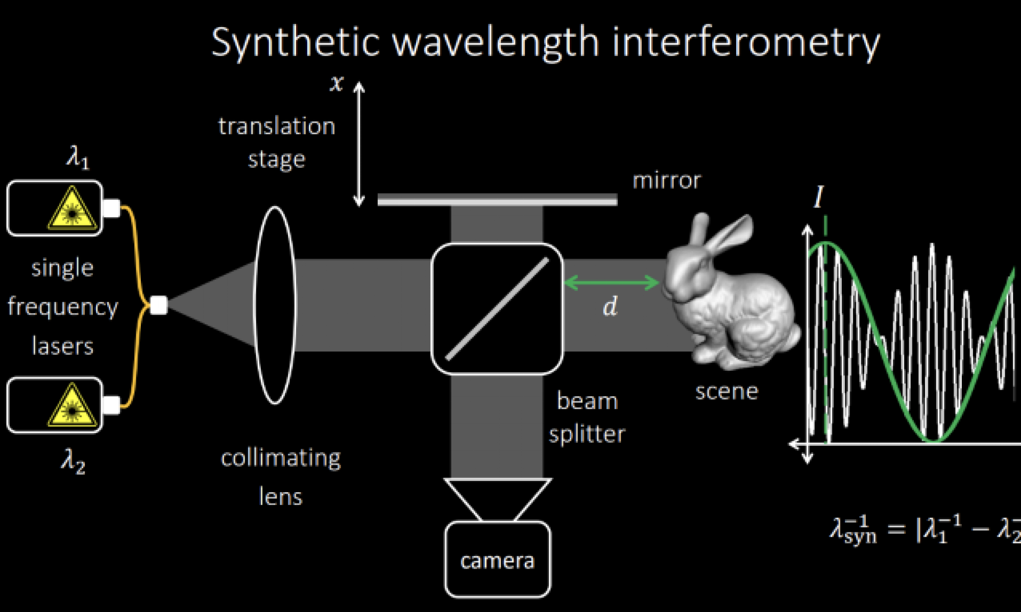
The technical name for this method is Synthetic Wavelength Interferometry. We aim to account for noise in the system using machine learning.
We pass two wavelengths instead of a broadband source. We get the intensity of pixel varying with mirror distance x like the white curve in Figure 1 .

If you’re familiar with amplitude modulation, there is a carrier wave which is high frequency and there is a message wave (green curve in Figure 1) which defines the amplitude.
Note that this green curve i.e. the message peaks at x = d + (n * wavelength) where d is the depth and n is integer
Using amplitude demodulation or carrier removal described below, we are able to get what measurements on message wave would look like. Assume for now, we need 4 measurements at predefined locations on the message wave to get depth.
Intuitively, to get 1 message wave measurement at some location, we take 4 measurements close to each other around the desired location. The gap between the 4 measurements is such that we cover one oscillation of high frequency carrier wave. See Figure 2
Since carrier is high frequency, we can assume the amplitude changes due to the message wave for let’s say the 4 blue measurements(in Figure 2) is negligible. We can just take the norm of the 4 measurements to get the amplitude.
We take 16 measurements as shown in Figure 2 to get 4 message wave measurements.

We now have 4 measurements of the message wave at our predefined locations.
Assume through some math, preprocessing and defining our measurement locations intelligently, the 4 message wave measurements for a given pixel p for our purposes represent [cos(d), sin(d), -cos(d), -sin(d)] where d is depth*2pi /wavelength. But you can think d is depth since scaling factor of depth is known and therefore irrelevant. And all depths for our analysis are angles which can be scaled using a known scale to get millimeters
Note that we get same 4 measurements if d was d+2pi . This means we can only measure depth uniquely if we knew for a fact that our entire scene is between 0 and 2pi. The reason my initial approaches in this project didn’t work were because this assumption of constraints on depth was not true for our dataset. While our scene had max depth – min depth <= 2pi, there was no guarantee that min depth wasn’t negative. Since we constrained any extracted depth to be between 0 to 2pi, the negative d‘s get mapped to 2pi +d . This would also happen if max depth was greater than 2pi.
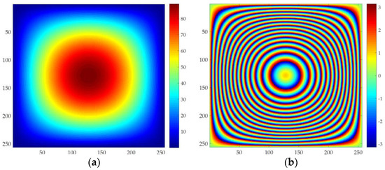
The above effect is called phase wrapping. The below image demonstrates it.

Note that in above example scene has much larger variations in depth that our dataset, thus more nested contours.
Assume that there exists phase unwrapping algorithms to get depth from phase wrapped depth.
Our contribution in this work is as follows, we tried following approaches
- Training a model which takes measurements and gives us a depth . We compare output depth to match ground truth depth.
- We simply convert our ground truth depth to what the ideal 4 measurements would look like and train the model to denoise our measurements to match the ideal measurements.
The first model would have to model inverse trigonometry and then take care of modelling phase unwrapping whereas the second model only has to worry about removing noise in our sensor data. We can do inverse trigonometry and phase unwrapping on top of the clean measurements our model gives.
A small detail in 2nd solution is to use a per-scene shift parameter for depth before converting ground truth depth to ideal measurements. This parameter is trainable and accounts for any shift in depth across the two methods. Another thing is we maximize the dot product of ideal measurements HxWx4 and clean measurements HxWx4 along the last dimension instead of taking an L2 loss.
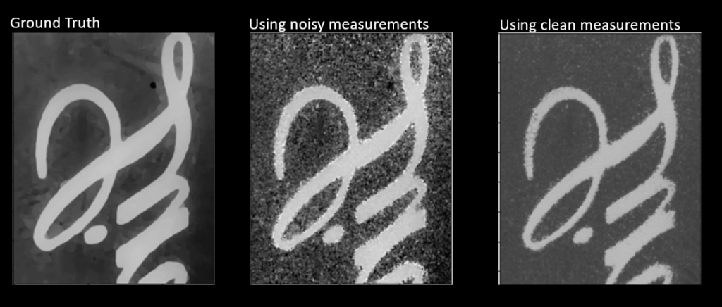
Results(trained for very few epochs and small network)

Error RMSE
Using noisy measurements : 0.0314 mm
Using clean measurements : 0.0257 mm
