As discussed in the Supervised Learning section, we are able to learn a quadtree/octree with supervised learning. However, results show that the supervised learned model has a hard time interpolating the testing space. This urges us to switch to a learning scheme that is more suitable for a quadtree/octree, Reinforcement Learning (RL).
Reinforcement Learning (RL)
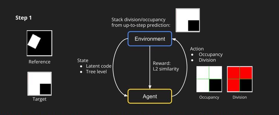
Reinforcement learning (RL) is a learning paradigm popular for learning a sequence of decisions. In an RL algorithm, there is an agent (or called an actor) and an environment. See the figure down below.
Take chess playing as an example. Imagine you are the actor, and the environment is the chessboard that you are playing with your opponent. First, it starts with the environment outputting the empty chessboard as the initial state observation. Then, as an agent, we should decide on a play (an action) based on this observation. The environment (opponent) would take in the action, play his round, and output a new state observation. We iterate this process until someone wins the chess game. At last, the environment should give a positive reward if the agent wins the game, or give a negative reward if the agent loses the game. This is essentially what RL is trying to do: learning an agent to do a sequence of actions.

Formulating Our Problem as RL
How can we model our task to an RL task? We first simplify the problem. Similarly, we target creating a quadtree for a 2d image, but we put the RGB information aside and just predict the occupancy of each node. We can think of the dividing process at each level as an action that an agent makes. In the first step, to predict a quadtree of tree level 1, the environment first gives the agent a state including a latent code and a tree level. The agent is going to predict the occupancy and division at the first level. The environment then can render an image based on the prediction and a reward which we set to be L2 similarity between the target and rendering.
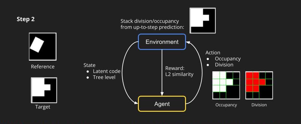
Then, we enter the next step. Given the state by the environment and knowing what are the division nodes, the agent will predict the occupancy and division for tree level 2. Again, the environment can render the images of level 2, combining the prediction from tree level 1 up to the current level.
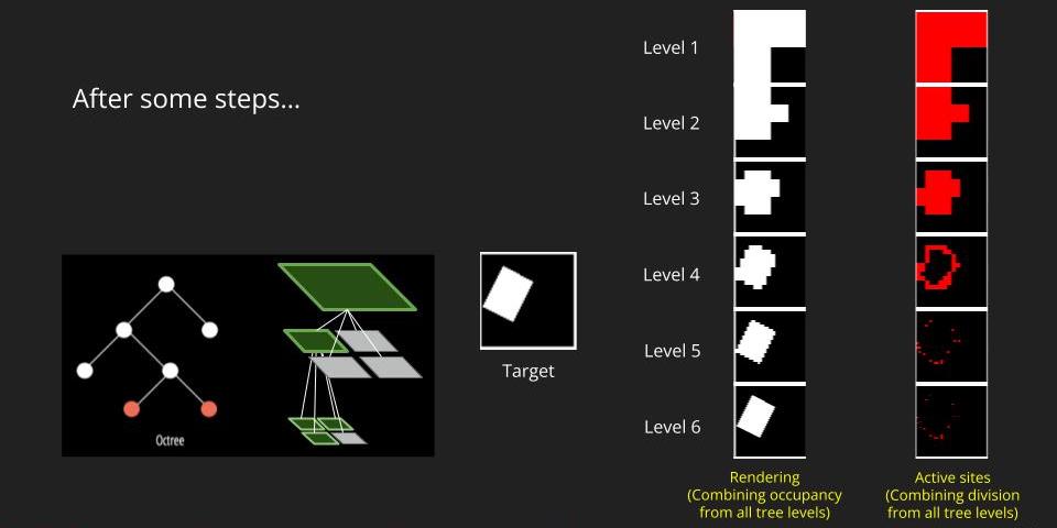
We repeat this process all the way to the target level. The figure below is what we expect to get. The active sites at each level means the nodes that we keep dividing. The idea active sites locate at the boundary of the object because those are where need a deeper tree level to represent the finer structure. To get the rendering at each level, we combine the occupancy of all levels.
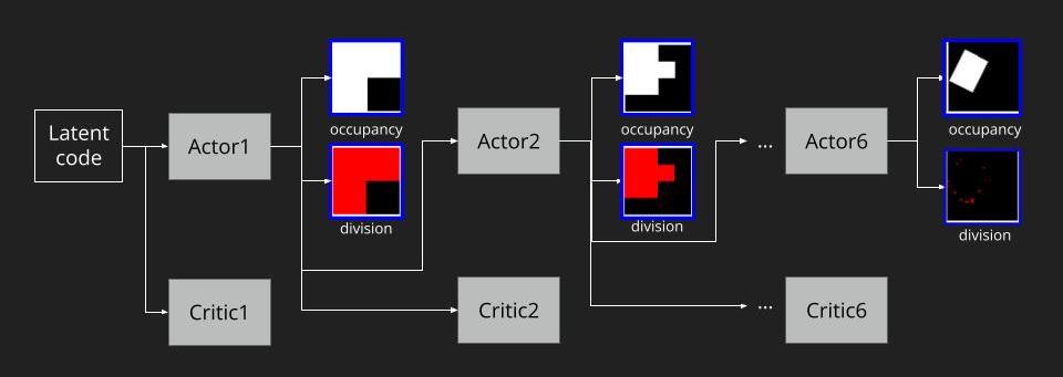
To understand the full RL process, we can roll out the steps as the figure below. As we follow A2C to train our model, we pass the latent code to the step-1 actor and step-1 critic to generate occupancy and division at tree level 1. The feature from step-1 actor would pass to step-2 actor and critic to continue the tree level 2’s prediction. All the way down to the target tree level. Note that these actors of each level do not share parameters, and neither do the critics.
As for the reward, the final reward design is:
Reward = L2 similarity + SSIM similarity – Node amount penalty
The first 2 terms encourage the actors to jointly predict a good rendering that can reconstruct the target image. The last term serves as a regularization term to limit the number of nodes grown in the quadtree. The reason to add this term is that without this regularization, we find the model tends to overgrow the quadtree, which means to divide the whole image into the finest resolution then predict the occupancy.
Implementation detail
We follow the A2C formulation (a variant of policy-gradient RL) to train our model. For each actor, we use an up-convolution to extract features and increase resolution. Then we employ two convolution branches to predict occupancy and division. As for the critic, we stack several convolutions followed by an average pooling layer to obtain the value prediction of the states.
Some other implementation detail
One thing to note is that we actually use an encoder to obtain the latent code for the initial state of RL. We realized that handcrafted latent code is difficult for a neural network to reconstruct the target. To ensure that the latent code has enough information encoded, we use a fixed pre-trained encoder (from a pre-trained autoencoder) to encode the target image into the latent code. We use multiple layers of convolution as our encoder.
Also, since the RL model takes a long time to converge, we adopt a progressive training strategy to accelerate the convergence. In the first stage, we train step-1’s actor/critic. In the second stage, we use the weights from the first stage as the pre-trained weight to initialize step-1’s actor/critic, and train step-1’s to step-2’s actor/critic. This process is repeated until the final step.
Results on 2D data
We first test our idea on the 2D data. The data is similar to what we use in the supervised learning section. We render a random rectangle in a 64×64 image. Then we ask our RL actors to reconstruct this rendering by predicting a quadtree.
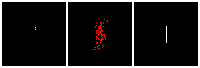
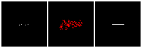
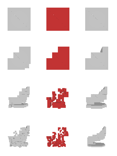
The rendering result of each tree level (step) is shown below. We can see the rendering improves as the tree grow more levels. The final rendering could well-reconstruct the ground truth image (shown by GT). One thing to note is that the active sites first focus on the entire occupied region, but as it grows deeper into the tree level, the active site focus on the boundary of the occupied region. This corresponds to what a reasonable quadtree should do: Only divide at places where fine detail is.
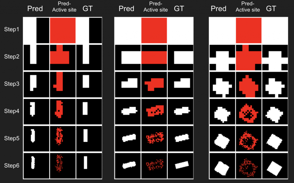
The next thing is examining the interpolation ability of our proposed RL method. Similar to what we did in the supervised learning section, we interpolate rectangles of different locations, scales, and rotations, all within the testing space, and ask the network to reconstruct it.
Results are shown below. We could observe that the trained RL actors could perfectly render the interpolated images. This indicates that our actors have the ability to predict tree structure for images that it has never seen. This is contrary to supervised learning. We attribute this to the fact that the RL learning paradigm let the actors learn to explore different tree structures to render, instead of restricting to a single ground truth tree.


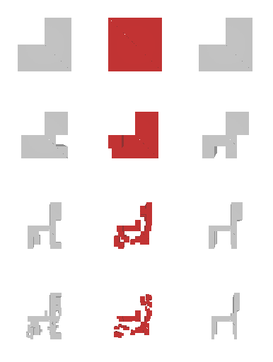
Results on 3D data
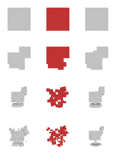
Next, we validate our method on 3D data. The data we use is from R2N2 dataset. We use a subset of the “chair” category to train and test our method. We ask the network to reconstruct 32x32x32 voxel representation of chairs.
Results are shown below. While the method could reconstruct results of just-ok quality up to level-3 (step-3), it produces a pretty poor result at level-4 (step-4). This indicates that the step-4 actor is not performing well. We speculate that this is because, at step 4, the action space is getting really large, approaching 2^4096 possible actions to perform to be exact. RL algorithm has a hard time figuring out which is the better action to make at this scale of action space.
Conclusion
In conclusion, we propose to formulate the quadtree/octree prediction as an RL problem. Results show that it could perform well on 2D data, but still room for improvement for 3D data. We also show that this kind of method is performing far better than the previous supervised learning method. Still, how to constrain the action space of RL is the critical future direction for predicting octrees on 3D data.