This project was conducted from Jan 2020 to Dec 2020, as part of the Capstone Project for the MSCV program at Carnegie Mellon University and also sponsored by Facebook Reality Labs (FRL).
Professor Srinivasa Narasimhan of CMU RI and Shoou-i Yu, He Wen of FRL participated in this project.
Motivation
Up to this point, research on human poses were only focused on certain keypoints, such as the joints.
However, human joints are not enough to create a dense 3D avatar of a human.
Preferably, a compact mesh of the entire surface of the body would be needed to do such a task.
In order to create a mesh, we would need to know as many locations of surface points as possible.
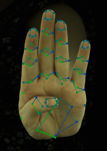
We need more keypoints other than human joints, such as points on the surface of the body. Hands are a key component of human communication. Hand gestures often play a key role in helping face-to-face verbal communication. However, hands are very difficult to detect, because they are small compared to the body. Also, they are often partially or wholly occluded. Nevertheless, it is crucial that we are able to detect dense hand keypoints.
Goal
In this project, we have the following goals:
1. Given 2D sparse keypoints from multiple view, predict 3D dense keypoints. (Spring)
– Key challenge: our 2D dense keypoint dataset is very small, and also every items does not have the complete set of dense keypoint labels.
2. Given a 2D monocular image, predict 2D dense keypoints. (Fall)
– Key challenge: like goal 1, our 2D dense keypoint data is very small. Also, we utilize generated labels (pseudo-labels) and use this data to train our network. Our network must learn to not overfit to these incorrect pseudo-labels and generalize well.
Dataset
In this project, we utilize two datasets:
1. Sparse + dense hand keypoints (non-public)
2. InterHand2.6M [link]
3D Dense Keypoint Detection from multi-view images (Spring)
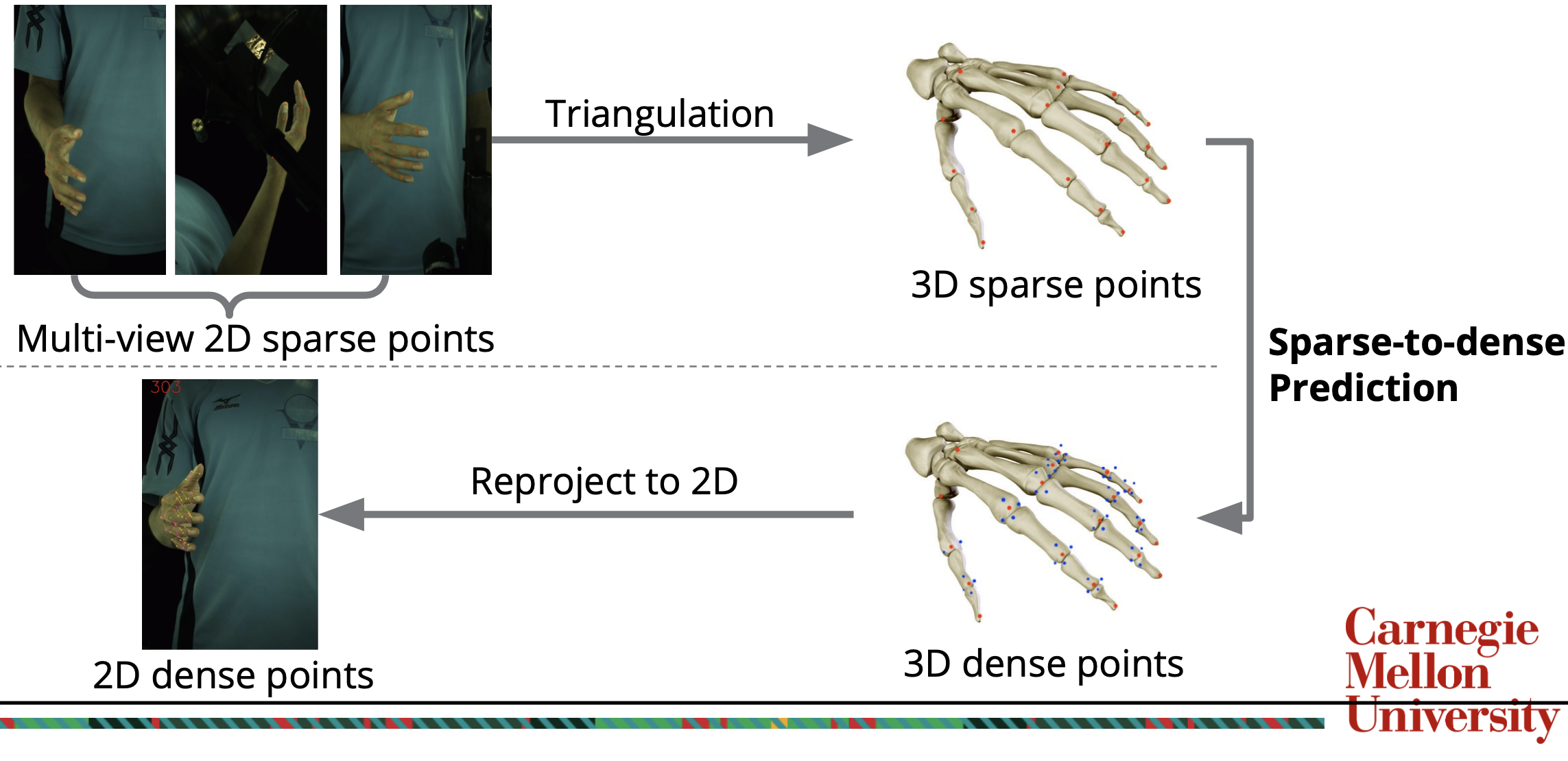
In our dataset, we have a small set of labels of 2D sparse and dense keypoints from multiple view.
Using these labels and camera intrinsics/extrinsics, we first triangulate 2D sparse/dense keypoints to 3D sparse/dense keypoints.
We then train a neural network to input 3D sparse keypoints and output 3D dense keypoints and the confidence scores that they are within the image.
Our loss function consists of the localization loss and a confidence loss.
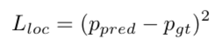
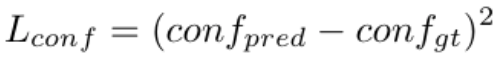
The localization loss is a simple mean square error (MSE) loss, and the confidence loss is a cross entropy loss.
After such a network is trained well, we can output 3D dense keypoints for any set of 3D sparse keypoints.
With these predicted 3D dense keypoints, we can reproject the coordinates into 2D with camera intrinsics/extrinsics to finally obtain 2D dense keypoints.
We build two versions of the network for 3D dense keypoints prediction: Rotation-to-Caging Network 1.0 and 2.0 (RTC 1.0 and RTC 2.0 in the following table):
1. RTC 1.0 : The network output is all 64 dense keypoints on one hand.
2. RTC 2.0: The network output is only one dense key point on the hand and there would be in total 64 models for 64 dense keypoints.
Our following quantitative experiment shows that RTC 2.0 performs significantly better.
| Training Method | Normalization and Augmentation | Average distance between prediction and ground truth |
| RTC 1.0 | Yes for both | 3.99 mm |
| RTC 2.0 | No for both | 3.66 mm |
| RTC 2.0 | With Augmentation but without nomalization | 2.42 mm |
| RTC 2.0 | Yes for both | 0.95 mm |
| Goal | < 2.00 mm |
Demo videos from multi-view images can be found here.
All of the three columns’ detected keypoints were generated from multi-view images, so there is no discrepancy between the keypoints generated for each view.
Monocular 2D Dense Keypoint Detection (Fall)
With our work in the spring, we were able to create a new dataset with pseudo-labels by predicting 2D dense keypoints from the InterHand2.6M dataset.
With this pseudo-label dataset, we have trained a monocular 2D dense keypoint detector.
The model was based on Convolutional Pose Machines.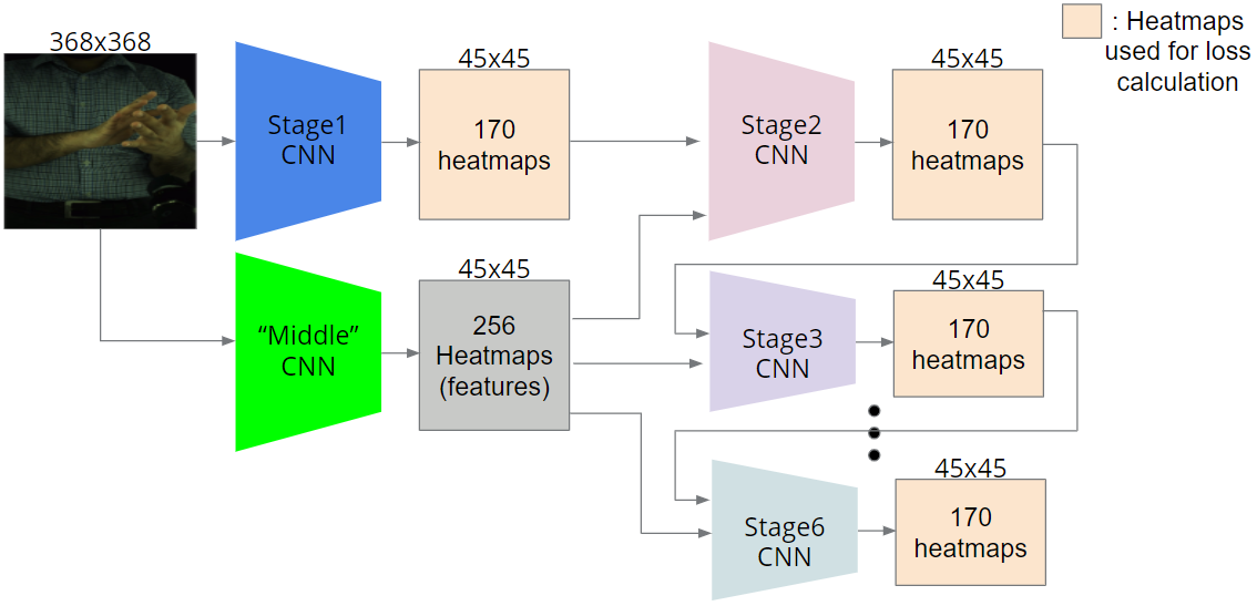
In essence, the model predicts heatmaps of the 170 sparse+dense keypoints, and in the following stages, it uses this information along with image features to predict better heatmaps.
CPM’s loss is defined as follows. For each stage t
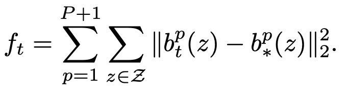
where p is the index of the keypoint and b denotes the corresponding belief map(heatmap, predicted and ground truth).
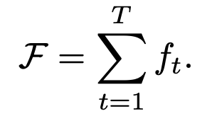
and the loss for the whole model is
We also build two version of model:
- CPM based model
- A model based on ResNet34 which does not include the heatmap prediction. (Directly regress on the L2 distance between ground truth locations and predicted locations)
Here is the quantitive comparison table (Average error measured in pixel with the image size of 224 x 224). Results show that CPM based method demonstrate a better generalization ability.
| Train set error (one hand image) | Train set error (two-hand image) | Test set error (one hand image) | Test set error(two hand image) | |
| ResNet 34 based method | 1.10 | 5.79 | 1.13 | 9.81 |
| CPM based method | 3.02 | 3.62 | 7.75 | 8.64 |
To generate 2D coordinates(334 x 512 or 512 x 334) from heatmaps (45 x 45), we need an upsampling method.
In most recent works, bicubic upsamling is a popular way of doing this.
However, we have found that this leads to a loss of information and consequently, more erroneous results.
Therefore, we take a 5 x 5 patch centered on the peak in the heatmap, and calculate the weighted average. With this weighted average, we upsample it to (w x h) by multiplying the x coordinate by (w/45) and y coordinate by (h/45).
Demo videos on monocular images can be found here.
Each of the three columns’ detected keypoints were generated from only monocular images, so there may be a discrepancy between the keypoints generated for each view.