Overview
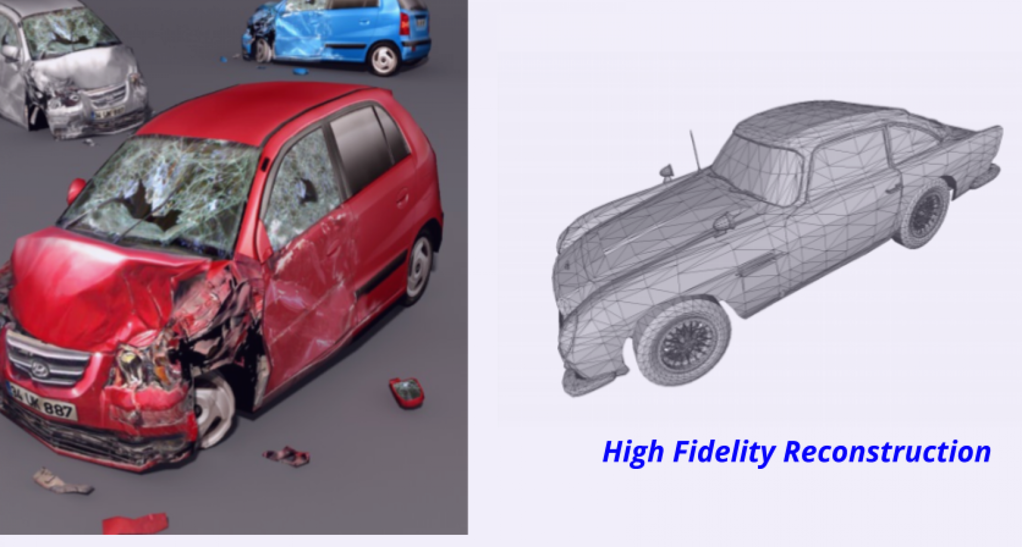
The primary goal of this project is to achieve high-fidelity 3D reconstruction by learning implicit representations. In contrast to the existing literature, we aim to design a method that can be used to learn these representations for any arbitrary shape, be it open/closed, or shapes which have ill-defined genus. The applications of this method include high-fidelity reconstruction of damaged vehicles for insurance purposes, and automatic computation of building roof surface area via 3D reconstruction from aerial imagery.
Project is Sponsored by Verisk Analytics and advised by Prof. Laszlo Jeni at CMU and Dr. Maneesh Singh from Verisk.
Approach
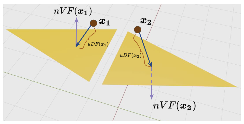
We disentangle the implicit representation of a shape into an unsigned distance field uDF and a normal vector field nVF. This decomposition enables us to represent both open and closed shapes with arbitrary topology, which, to the best of our knowledge, is a significant improvement over existing methods. We aim to model these functions using feed-forward networks with non-linear activation functions.
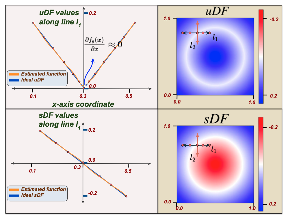
We begin with a formal definition of a uDF: it’s a function that outputs the closest unsigned distance to the surface from any given point in 3D space. Note that this is in contrast to an sDF which is meant to output negative distances inside the shape and positive distances outside. Several notable current approaches for representing shapes, thus bound to the assumption that the underlying surface is watertight. We argue that an sDF can inherently describe only closed shapes. To relax this assumption, we model a 3D shape using a uDF which can represent both watertight and non-watertight shapes equally well.

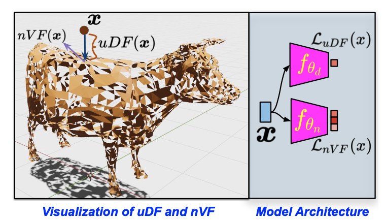
As can be noted, trivially removing the sign of the sDF leads to a uDF. However, this sacrifices some important properties of the sDF leading to a new set of challenges which we need to address. (1) The uDF is non-differentiable at the surface (see Figure 2) implying it can’t be reliably trained using points sampled from the surface. We overcome this by never actually sampling the training data points on the surface but slightly away from the surface; (2) Unlike sDFs, we cannot reliably extract the surface normal from a uDF due to its non-differentiability (See Figure 2). Since estimation of high quality surface normals is important for several downstream tasks, we propose to learn a normal vector field (nVF), which, for any 3D location, 


Given a 3D shape represented by the noisy triangle soup, we construct training samples, 


We first densely sample a set of {points, surface normal} pairs from the triangle soup, by uniformly sampling points on each triangle face. Let’s call this set of points $ latex \mathcal{X}= {(\boldsymbol{x_s}, \boldsymbol{v_s})}$. Since each point is sampled from a triangle face, the normal to the triangle face provides the associated surface normal for that point.
Given this set $ latex \mathcal{X}$, the set 


Before we describe how 


This allows for the network to learn surface normals
Sphere Tracing uDFs
Sphere tracing is a standard technique to render images from a distance field that represents the shape. To create an image, rays are cast from the focal point of the camera, and their intersection with the scene is computed using sphere tracing. Roughly speaking, irradiance/ radiance computations are performed at the point of intersection to obtain the color of the pixel for that ray.
The sphere tracing process can be described as follows: given a ray, 


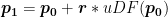

![[\boldsymbol{p_0}, \boldsymbol{p_1}]](https://s0.wp.com/latex.php?latex=%5B%5Cboldsymbol%7Bp_0%7D%2C+%5Cboldsymbol%7Bp_1%7D%5D&bg=ffffff&fg=000&s=0&c=20201002)


Note that for uDF, the above procedure can be used to get close to the surface but doesn’t obtain a point on the surface. One we are close enough to the surface, we can use a local planarity assumption (without loss of generalization) to obtain the intersection estimate. This is illustrated in Figure 4 and is obtained in the following manner: if we stop the sphere tracing of the uDF at a point 

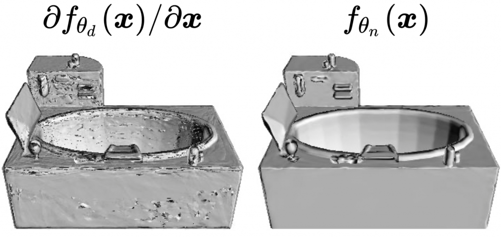
Benefit of using nVFs
In Figure 5, we visualize ray casting using normals obtained by differentiating the uDF (Left) and ray casting using the surface normals estimated by the nVF (Right). This high-quality rendering empirically validates the need for learning an nVF alongside a uDF.