Abstract
TODO
Method
Classical Stereo Depth Estimation
Depth estimation using stereo is a well-researched area and has many different approaches. The classical methods for stereo depth estimation are fairly straightforward and don’t involve any learning or need for data. These methods consist of the following steps:
- Extracting features from both images.
- Construct a cost volume that captures how the left and right feature maps match each other on different disparity levels.
- Using epipolar geometry, calculate disparity from the computed cost volume. (Looking for which disparity has the highest confidence)
The main limitation of the classical stereo methods is that they are limited by the handcrafted features extracted in the first step.
Learning Based Stereo Depth Estimation
Several different architectures have been proposed for stereo depth estimation using CNNs. PSMNet. Given two images, each image is first fed through the same encoder which creates image features. Then these image features are compared to each other to construct a cost volume where for each pixel there is an associated probability distribution over a set of discrete pixels. Posing this as a classification problem results in issues with sub-pixel disparity errors. Instead, we use a typical regression loss function and try to minimize the error between weighted sum over the disparities and the ground truth disparity.
Deep Hierarchical Stereo Matching builds on top of PSM net and several other works to focus on specifically improving the performance on high-resolution images. Typical models would suffer with high-resolution images, however, deep HSM addresses these issues by using a coarse-to-fine strategy for depth estimation.
As shown above, deep HSM follows similarly to PSMNet using CNNs to extract image features for each image pair. However, a key difference is that Deep HSM retrieves the features at different resolutions. Each resolution feature map is matched with each other to create a 4D cost volume. In the decoder, 3D convolutions are applied to get a disparity map for the given resolution, as well as a new cost volume to bias the next finer resolution. Overall, Deep HSM is able to perform much better on higher resolution imagery by following this coarse to fine strategy.
Domain Adaptation
One possible solution for low-light stereo is using supervised learning methods trained on low-light/night-time data. However, obtaining proper disparity ground-truth data that is dense and independent of glow or flare is extremely difficult.
Domain Adaptation is the ability to apply an algorithm trained in one or more source domains to a different target domain. In our context, we tried to use this technique to leverage the existing daytime data(along with daytime ground truth) to learn a low-light/night-time stereo model. The primary challenge here is that the input images have some geometric consistency which might not remain when passed individually through domain adaptation networks. In the example below, when converting a stereo pair from synthetic to real, we see that the resulting images have new artifacts introduced that are not consistent:
Add stereo inconsistencies image
Our method uses a CycleGAN architecture to change from daytime to nighttime and vice versa. Below is the architecture diagram for this method:
Add architecture image
The key contribution of this method is the way in which consistency is maintained in the generated images. This is called the structure-consistency constraint and is enforced by a structure preservation loss. This loss is based on the idea that the features obtained from the input image pair should be similar to those of the rendered image pair. A pre-trained VGG-16 is used to extract these features. Given an input night pair (xln , xrn) and the corresponding rendered night time image (zld , zrd), we can define the structure preservation loss as ,
Add equation
Where 𝜙 denotes the VGG-16 feature extraction function.
Here are a few results obtained from this methods:
Add conversion and stereo results
The limitation of this method is that the domain gap between day and night time images is too huge to be covered by a single model. In cases where the input image is extremely dark, the rendered image is extremely noisy. To overcome this, we considered the use of an intermediate domain to reduce the domain gap.
Thermal Based Stereo
Another modality that we considered using is thermal images. The advantages of using thermal cameras are that is is passive and is mostly unaffected by lighting. Thermal data can also be used for domain adaptation as the gap between day and night thermal images is much smaller than the gap between day and night RGB images. We are looking to explore more in this domain next semester.
Evaluation Metrics
We use standard evaluation metrics listed below from KITTI and Middlebury datasets.
- Average Error – The average error between ground truth disparity and predicted disparity over the entire image and dataset.
- Bad-X Error – The percentage of pixels in the entire image which have an error > X in disparity.
- D1-All – This metric is used in KITTI Stereo Evaluation challenge and is equivalent to Bad-3 Error.
Confidence
Confidence metrics provide additional context to downstream components which can utilize the information to act accordingly. For example, a motion planner may avoid the high uncertainty in a particular region compared to highly-certain regions. We use entropy as one such metric that provides uncertainty information for our predicted disparity map. Specifically, we calculate the entropy of the discrete disparity probability distribution for each pixel.
In addition to entropy, we are also interested in potentially predicting confidence from the model directly. Several works have tackled this problem which has led to an improvement in performance, which we hope to reproduce in the near-future.
Experiments
Traditional Stereo Datasets
Due to the difficulty of getting labeled ground truth depth estimates, there are only a limited number of datasets. The most popular ones are KITTI, Middlebury, and ETH3D. However, these datasets are almost entirely focused on daylight with very few low-light environmental conditions.
Oxford Robot Car
Contains a large number of outdoor driving around Oxford at day and night time, as well as various weather conditions.
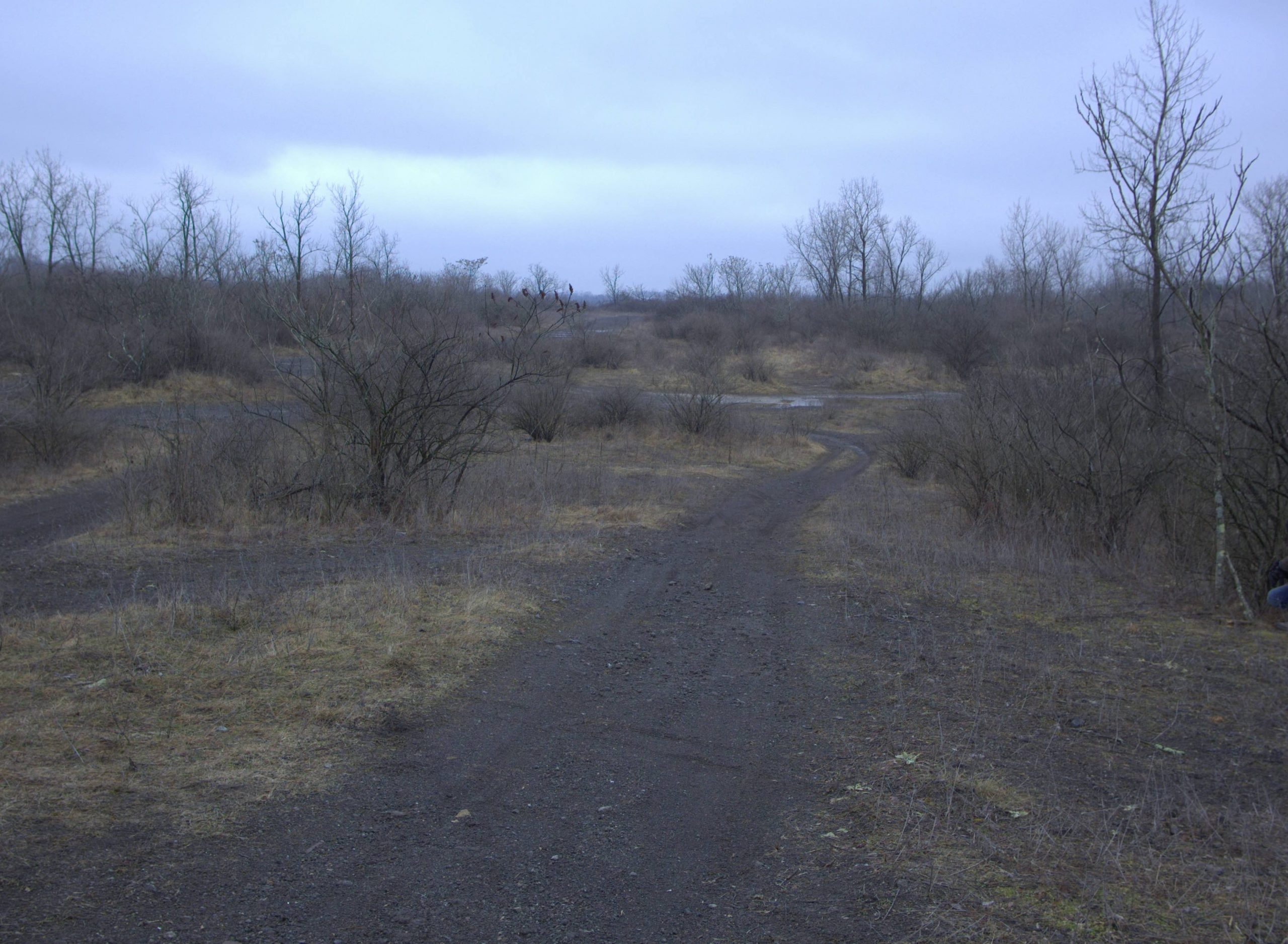
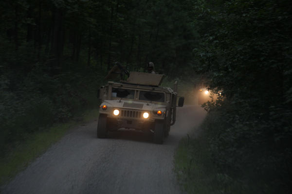
NREC Collected Data
The above datasets, while may be helpful to some extent, are certainly not in the same domain as the environments for our targeted application. Mainly, our environment contains not just low-light but also off-road environments for which there aren’t any publicly available datasets yet. As such, NREC has collected their own data at various locations that are closer to our actual domain. An example of one such locations during day-time is shown.