Introduction
Our project is about Millimeter-wave Radar SLAM. The goal is to build a SLAM pipeline for an extremely noisy Radar sensor. For the front-end part, we rely on a machine learning model to simultaneously estimate relative motion and extract plausible landmarks from sensor reading. For the backend part, we use odometry and landmark measurements from the front end to set up a pose graph and solve it with iSAM2 algorithm.
Weakly Supervised Keypoint Learning
There are some methods already existing for the odometry part of radar SLAM. However, they mostly rely on handcraft feature detectors. We have implemented one of them and tested it on our targeted dataset. The conclusion is that radar response is usually noisy and hand-designed features usually don’t generalize across different datasets. Instead, we make use of machine learning to automatically learn useful keypoints from just relative motion between two frames as ground truth. The whole network architecture looks like this:
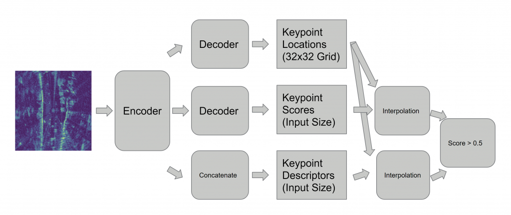
There are three branches for our keypoint detector. It takes the 2D radar response (bird’s-eye view of the street) as input. The first branch divides the input into a 32×32 grid, and outputs one keypoint location per cell. This is to ensure that the keypoints are well separated. The second branch outputs a keypoint score map for each pixel. The third branch outputs a keypoint descriptor map for each pixel. Then we can use the coordinates from the first branch to do interpolation to get corresponding confidence scores and descriptors. Finally we choose the keypoints that have score larger than 0.5.
We have just described the inference stage of our model. Now the training part is visualized below:
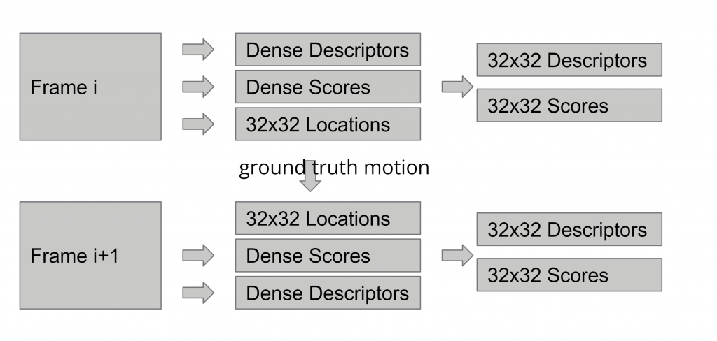
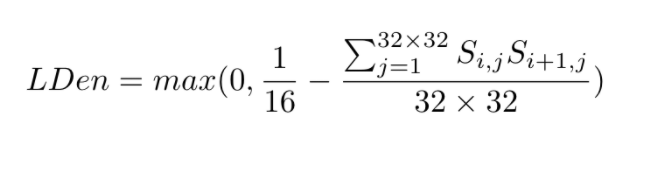
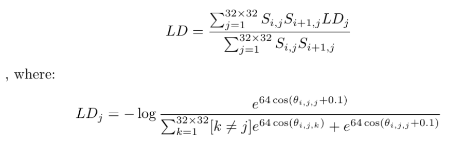
During training, we select two consecutive frames which have ground truth motion available. The model computes a set of keypoint information for each frame. Then we replace the locations of the keypoints of the second frame by the locations of they keypoints of the first frame transformed using ground truth. This ensures the correspondences of the two sets of keypoints. Then we compute a loss that measures how close the descriptors of the matched keypoints are, and use standard deep learning training techniques to optimize the model. We also incorporate a density loss the ensure that the confidence score of some keypoints are large enough. Our model achieves high-quality matching results and trajectories as shown below:
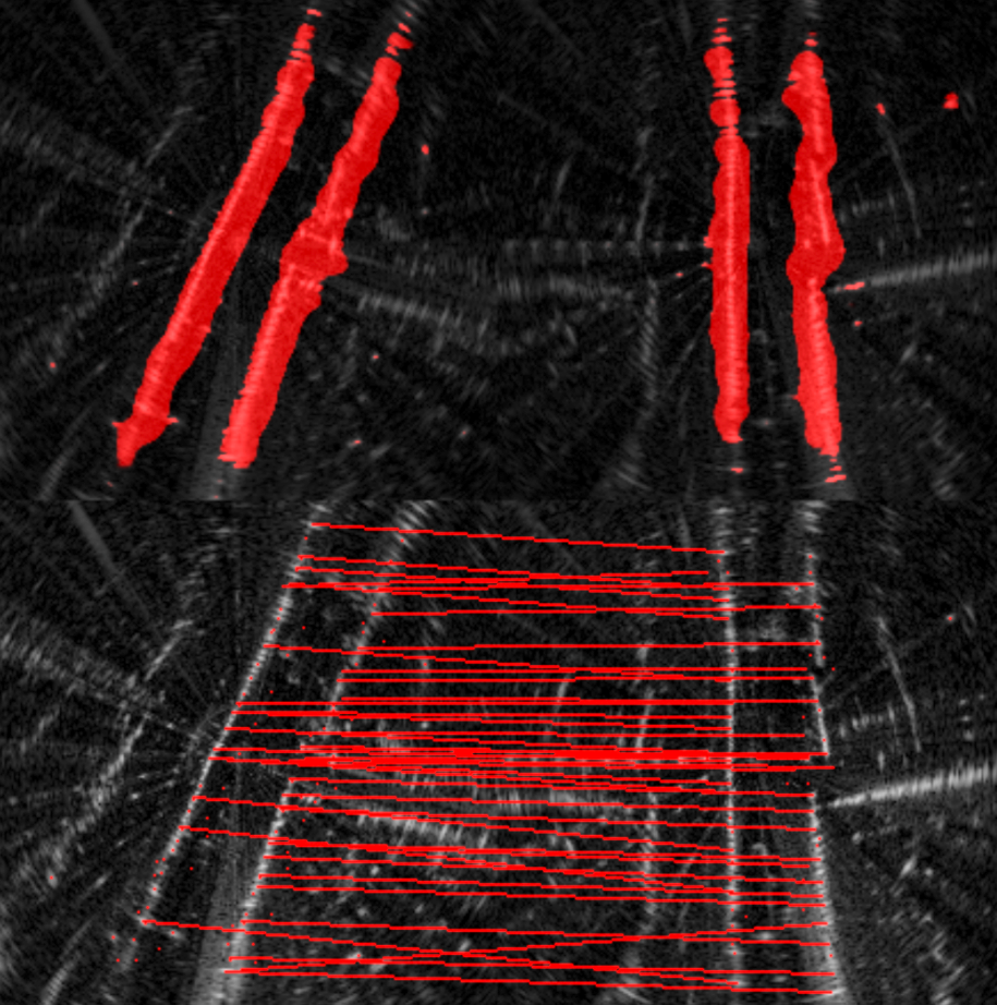
Keypoint Matching Result 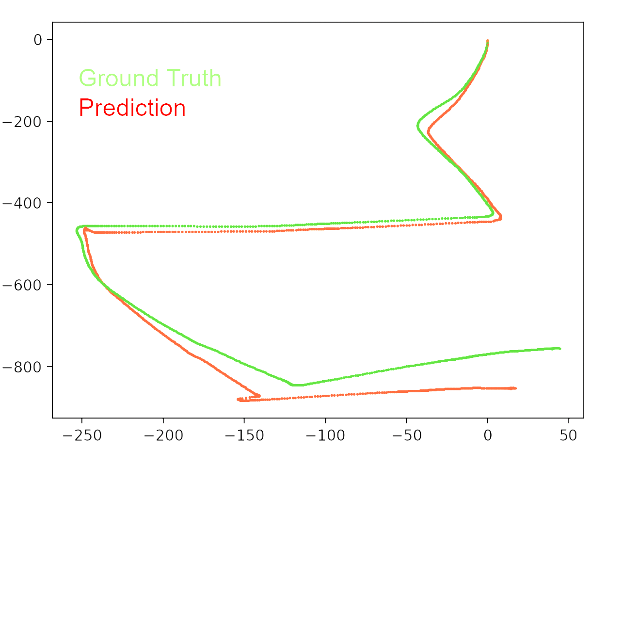
Trajectory
Point Cloud-Based Odometry
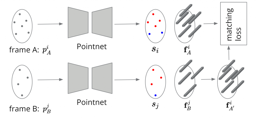
As for the 3D indoor dataset, we have developed a point cloud-based method for odometry. The idea is that we don’t want to waste memory and computation to process the whole space 3D volume. Instead, we select points that have high intensity values and use a point-based neural network call PointNet to compute the output keypoints and descriptors. However, the weakly supervised method would no longer work. So now we use lidar response as the additional supervision. This is possible because the dataset provides time-synced lidar response. We assign label of 1 to the radar points if and only if they are close to at least one lidar points. We also use the similar recognition loss to learn the descriptors:
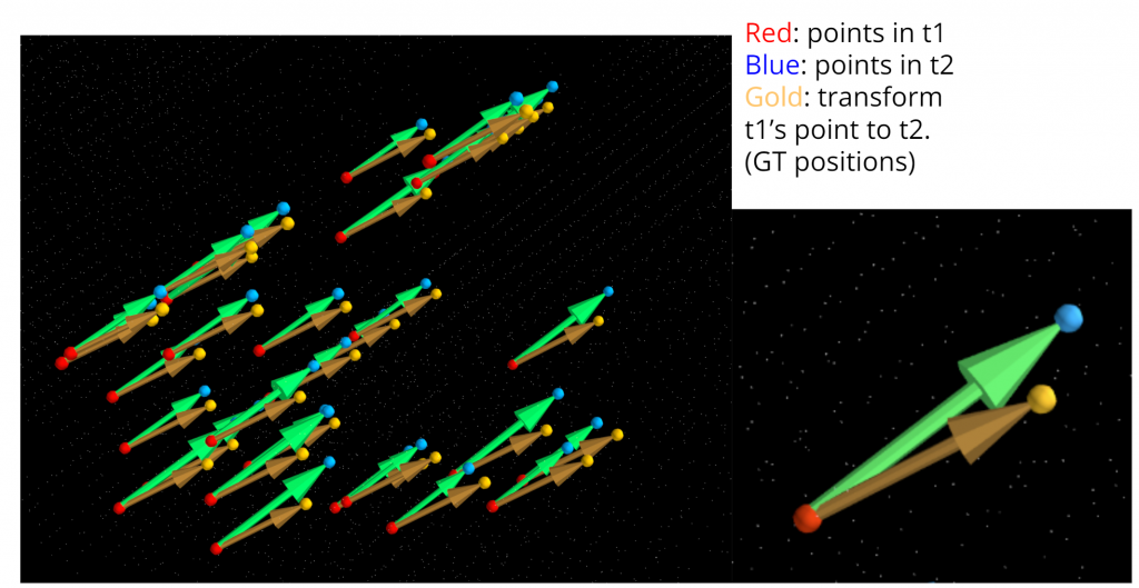
Our model predicts keypoint correspondences that are highly consistent and close to the ground truth. Although there is a small difference due to the fact that the resolution for the elevation angle is quite low.
End-to-end odometry
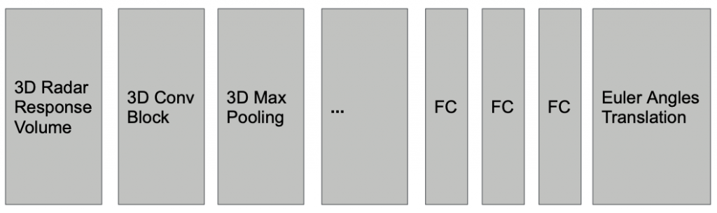
Motion Estimation: Since the discretization issue in point cloud based method is not trivially solvable, point cloud based methods will inevitably result in wrong motion estimation. We therefore take a step back to rethink about our pipeline. Since point-cloud based methods rely on the bound-to-be-noisy landmark detection result to estimate motion, is it possible to decouple motion estimation from landmark detection, such that motion estimation doesn’t have to deal with the discretization problem? The answer is yes, we can directly estimate motion from the raw radar data using a neural network. The input is the 3D radar response volume; the output is a 6-dimension vector with 3 for translation and 3 for Euler angle. An illustration of the network is shown below. Since it outputs continuous values, we consider it as a regression problem and use MSE as our loss function.
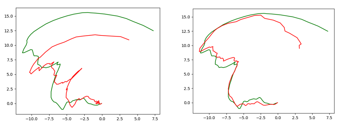
We found this model performs much better than point-cloud based methods in trajectory estimation. The image below compares trajectories from point-cloud based method and the direct motion estimation method. We can see that the latter performs much better than the precious one. The difference mainly comes from the discretization issue and landmark association errors in point-cloud based methods. The direct motion estimation method also utilizes the entire radar response volume for prediction, which contains more information than point cloud. But note that the new model requires more data than point-cloud based method, since we are not using any geometry knowledge to estimate motion but training a model to predict it. So it requires more data to learn the underlying geometry.
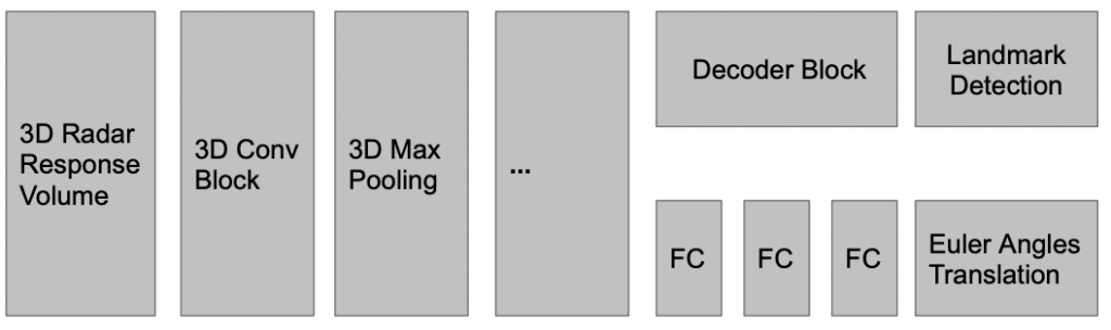
Landmark detection: We further extend it to perform landmark detection by adding a decoder on top of the backbone to predict the probability of each voxel being a true landmark. The label of each voxel is one if the LiDAR density around that voxel is higher than some threshold, otherwise zero. The architecture is shown below. The decoder consists of several 3D ConvTranspose layer and Upsampling layers. We use binary cross entropy loss to train the model along with the motion estimation branch.
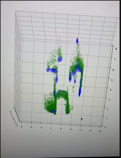
Here is a visualization of our landmark detection results. Green dots are landmarks detected over the past five frames, blue dots are landmarks detected in the current frame. We can see although not perfect, they are consistent over different frames and can be used for mapping.
Factor Graph Optimization
After obtaining motion estimation and landmark detection from each frame, we can plug them into a factor graph to obtain a globally optimized trajectory and map. The edge between two poses is the motion estimation from our model. The edge between a pose and a landmark is setup only when the landmark is consistent with the observation at that frame. Specifically, we project all map landmark to current local frame, and match them with the current observations. If a landmark is mutually matched with an observation and their distance is smaller than some threshold, we setup an edge between the landmark node and the current pose node. If an observation is far away from any landmark, we create a new landmark node and setup an edge as before. The following figures illustrates raw radar response, our construction of map and trajectory, and the ground truth.
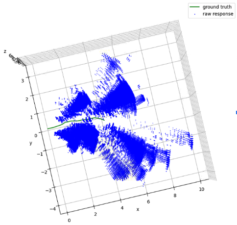
Input from radar 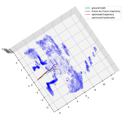
Our localization and mapping result 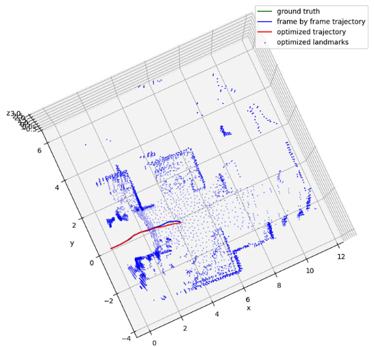
Ground truth
Advisor and Sponsor
Our CMU faculty advisor is Michael Kaess. We thank him for his essential guidance.
This project is also sponsored by Amazon Lab 126. We thank Jaya Subramanian from Amazon for her valuable advice.