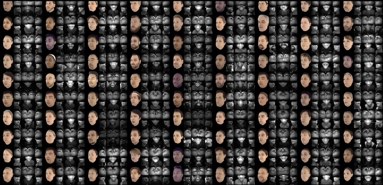

Dataset
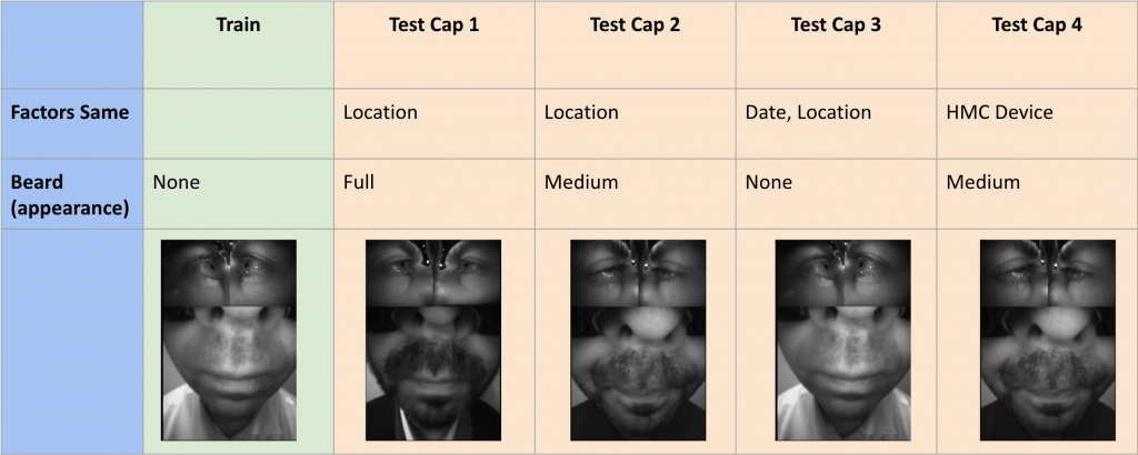
We have one capture that we train on and 4 captures for testing. The first row of the the table shows the factors that are common between the train capture and each of the test capture. The second and third rows show how the appearances of the subject differ between the captures.
Proposed Methods
Metric Learning
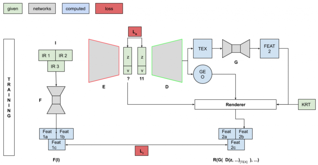
In this semester, we explored Metric Learning. The idea was to learn to transform input images and predicted texture to a generic feature space. We wanted a comparison in this feature space to minimize the distance between current code (3-view) to 11-view results and at inference, use this transformation to ‘refine’ the code using Gradient descent. This relies heavily on the assumption that 3-views have enough information to arrive at code 11-view. The diagram can be seen in figure. We want to ensure that loss is quadratic for fast gradient descent.
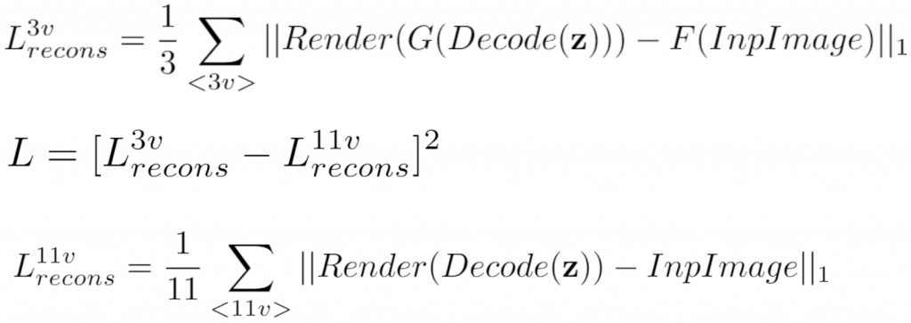
Mimicking the 11 View Landscape
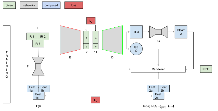
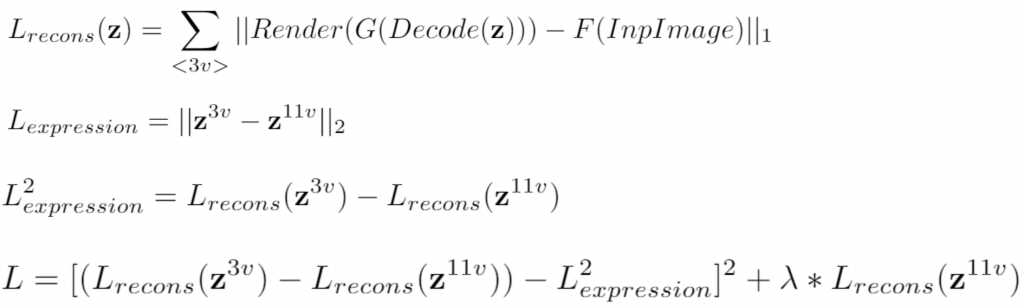
In this method, instead of ensuring that loss landscape is quadratic, we mimic the loss landscape of 11 view and the now it takes more time to gradient descent to correct expression and the losses are as follows.
Results
Metric Learning
In this method, instead of ensuring that loss landscape is quadratic, we mimic the loss landscape of 11 view and the now it takes more time to gradient descent to correct expression and the losses are as follows.
NOTE: If you do not see the video, please download and run it locally.
Mimicking the 11 View Landscape
In this method, instead of ensuring that loss landscape is quadratic, we mimic the loss landscape of 11 view and the now it takes more time to gradient descent to correct expression and the losses are as follows.