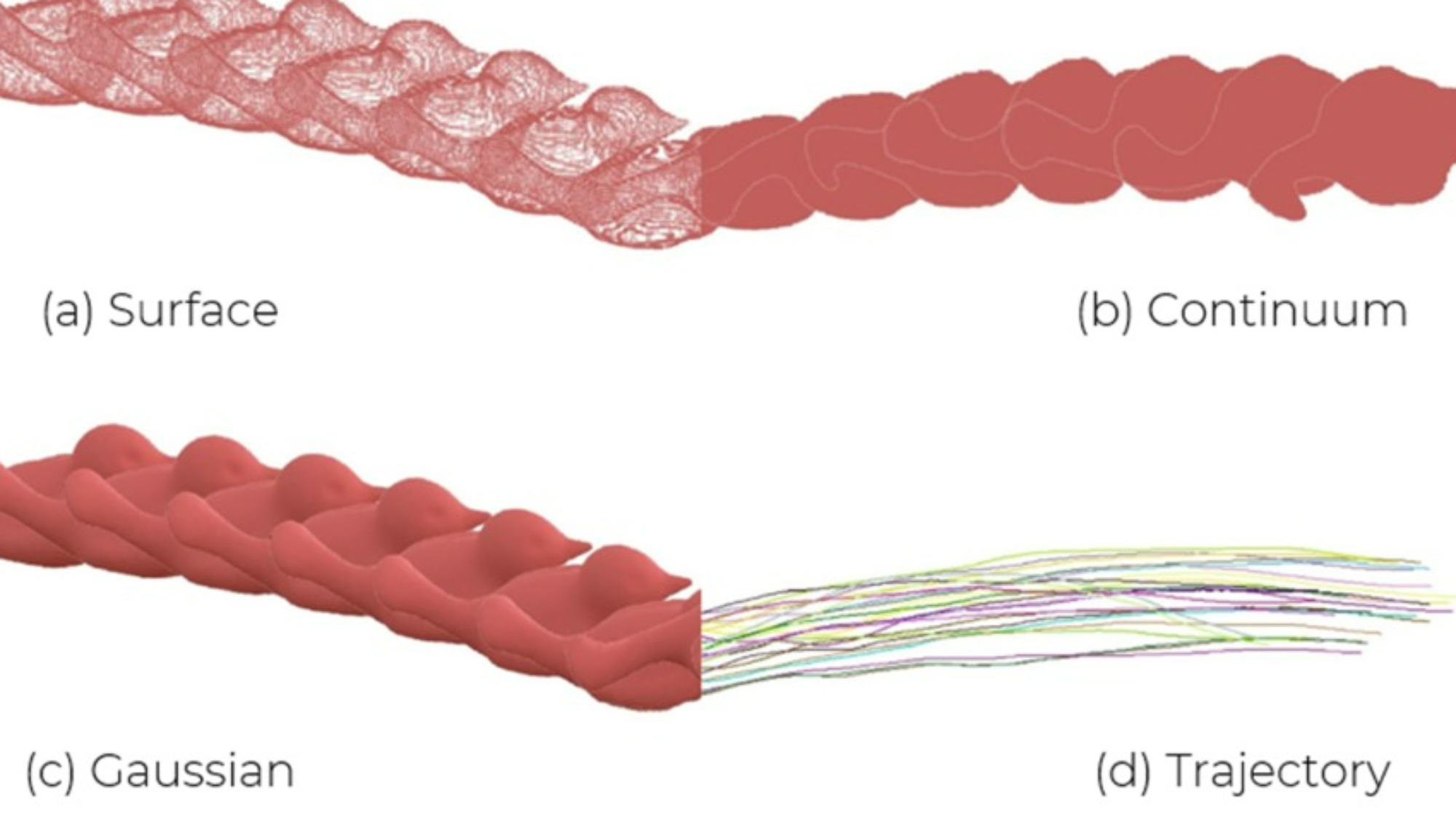
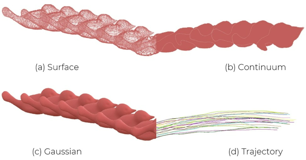
Our method is composed of two main steps. The first step is geometric reconstruction. Our algorithm utilizes four main geometric reconstruction targets: Surfaces, Continuums, Gaussians, and Trajectories. The second step is material-agnostic system identification, which parameterizes the object’s physical properties. Finally, with this parameterization, we can generalize to new scenarios.
Step 1: Geometric Reconstruction

Concretely, we follow previous works [1] in representing the object with 3D Gaussians [2] by maintaining a set of 3D Isotropic Gaussians with a center and scale. Then we train a deformation coefficient network that takes in the starting Gaussians and a timestep and outputs coefficients to transform them to the Gaussians at that future timestep.
These are optimized using the 2D rendered views following [2] with L1 and SSIM loss.

Since 3D Gaussian reconstruction is biased toward object surfaces, we must apply a filling procedure to initialize the starting particles of our object. To do so, we leverage the trained deformation network to predict the trajectories of the particles over time.

We fine-tune the network to do so using Chamfer Distance Loss against the ground truth point clouds.
This reconstruction process is repeated for all sequences of video data.
Step 2: System Identification
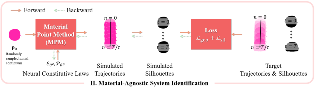
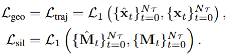
The second step is system identification. We train our model on multiple sequences of the same object with different initial conditions. At each training iteration, we randomly sample the initial continuum for one of the sequences, however, we use the same neural network to represent the physical parameters of the object in all sequences. This way, the network receives signal from all training sequences. Given the neural parameterization and initial continuum, the Material Point Method [3] simulates the trajectories of the particles through time. We also render out the object masks using the 3D Gaussians. This gives us our loss functions, which takes the L1 loss between the simulated trajectories and the trajectories obtained in step 1, and the L1 loss between the rendered silhouettes and ground truth object masks.
Multi-Object System Identification
In our next work, we follow our previous method for geometric reconstruction using 3D Gaussian Splatting. One difference is that instead of training a deformation network, we recover the simulation particles at each timestep by performing volume sampling on an increasingly fine density field at voxel locations inferred from 3DGS reconstruction. One key point is that we utilize additional labeled masks to perform this reconstruction on each object independently, so that we can assign independent material tags for each particle, ensuring material tags don’t get entangled during collision.
We utilize predefined expert constitutive models for our objects to model the response of particles based on the object’s physical parameters.

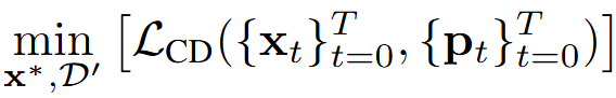
Similar to our previous work, a differentiable MPM simulation is rolled out on the objects and their initial parameters. During simulation, we can extract the particles and surfaces to optimize a geometrically and photometrically aligned objective:

Another key trick is that we gradually increase the rollout length as alignment improves, and interleave optimization with resynchronization of particle states, which helps us reduce any drift.
Having recovered the physical parameters, we can now undergo novel interactions with our objects!
References
[1] Junhao Cai, Yuji Yang, Weihao Yuan, Yisheng He, Zilong Dong, Liefeng Bo, Hui Cheng, and Qifeng Chen. Gic: Gaussian-informed continuum for physical property identification and simulation. arXiv preprint arXiv:2406.14927, 2024.
[2] Bernhard Kerbl, Georgios Kopanas, Thomas Leimkühler, and George Drettakis. 3d gaussian splatting for real-time radiance field rendering. ACM Trans. Graph., 42(4):139–1, 2023.
[3] Chenfanfu Jiang, Craig Schroeder, Joseph Teran, Alexey Stomakhin, and Andrew Selle. The material point method for simulating continuum materials. In ACM SIGGRAPH 2016 Courses, pages 1–52, 2016.