
SuperPoint & SuperGlue
The initial stages of bundle adjustment rely heavily on accurate feature detection and matching. To improve robustness and precision, we use SuperPoint, a deep learning-based detector and descriptor that identifies repeatable keypoints and produces distinctive feature embeddings. For the matching stage, we employ LightGlue, an attention-driven extension of SuperGlue that leverages global context to produce more reliable correspondences between feature sets. Since equirectangular images suffer from distortions that can degrade matching quality, we first decompose each 360° image into six perspective views, effectively creating a cubemap representation. Feature detection and matching are performed on these perspective images, and the resulting correspondences are then fed into a rig-based bundle adjustment framework, which enforces geometric consistency across all six views and improves the overall accuracy of the reconstruction.
Rig-Based Structure-from-Motion (SfM)

To handle 360° equirectangular images in standard SfM pipelines, each image is first decomposed into a cubemap, producing six perspective views. Although this increases the number of images sixfold, the six views are physically constrained relative to one another, allowing them to be treated as a single rig. By modeling the cameras as a rigid rig, we only need to optimize the rig’s global position and orientation over time, while the relative camera-to-rig extrinsics remain fixed.

The rig-based bundle adjustment jointly optimizes the following variables:
- Rig poses over time – the global translation and rotation of the rig at each timestamp.
- Camera-in-rig extrinsics – fixed relative poses of each camera in the rig.
- 3D point positions – spatial locations of observed scene points.
The optimization objective is to minimize the sum of squared reprojection errors across all observed keypoints:

- For every observed keypoint in a camera, the corresponding 3D point is projected into that camera using the current rig and camera extrinsics.
- The pixel-wise error between the projected point and the detected keypoint is computed.
- The optimization iteratively updates the rig poses and 3D point positions to minimize these errors, respecting the fixed camera-in-rig constraints.
This rig-based formulation allows existing SfM pipelines to handle cubemap decompositions efficiently, enforcing geometric consistency across all six views while reducing the number of free parameters compared to treating each perspective image independently.
Monocular Depth Estimation with Scale Alignment

We use a Monocular Depth Estimation (MDE) model to predict dense per-frame depth maps. Since monocular depth is scale-ambiguous, pre-trained off-the-shelf models cannot be used directly, as they need to be globally aligned with the scale of the scene and the detected 3D points. This approach first takes any pretrained model (ZoeDepth) and allows us to perform KNN and align the predicted depth to the sparse point cloud in patches (Explicit fusion). This densifies the sparse depth map into a complete yet inaccurate depth map (due to noisy points used during scaling). Once this alignment is done, a secondary prediction is made using the same prediction model, and a conditioned convolution network aligns local patch gradients to correct any discontinuities in the previously predicted depth, resulting in a final depth that’s scale-aligned with the point cloud.
GS for Unconstrained Photo Collections
We adopt Splatfacto-W, a variant of Gaussian Splatting specifically designed for unconstrained image and video collections captured in natural settings.

Simple 3D GS scene trained vs Splatfacto-W variant
Background: Original Gaussian Splatting
In Gaussian Splatting, a 3D scene is represented by a collection of 3D Gaussian primitives, where each Gaussian models a small region of space with its position (μ), covariance (Σ), opacity (α), and color (c). Unlike traditional point clouds or meshes, these Gaussians are continuous and differentiable, making them well-suited for gradient-based optimization.
3D Covariance and Projection
Each Gaussian’s 3D covariance matrix (Σ) defines its shape and spatial extent, modeling how much it influences the surrounding region. During rendering, this 3D covariance is projected into the 2D image space using a view-dependent transformation:

Here, W is the world-to-camera transformation, and J is the projection Jacobian, which approximates how the 3D Gaussian deforms when projected into 2D.
Color Representation and α-Blending
Each Gaussian carries a color (c) represented via third-order spherical harmonics, allowing it to capture view-dependent appearance (e.g., specularities and shading). The influence of a Gaussian on a pixel is computed using a 2D Gaussian function:
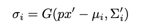
where σi is the contribution of the i-th Gaussian to the pixel at location r.
The final pixel color is computed using alpha blending,
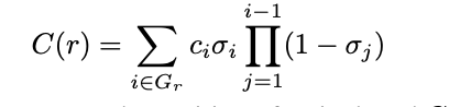
Here, r represents the position of a pixel, and Gr denotes the sorted Gaussian points associated with that pixel.
This blending process ensures smooth compositing and natural depth-aware rendering.
GS in the Wild
‘GS in the wild’ introduces three key innovations to handle real-world variability:
- Neural Color Fields
Each 3D Gaussian is assigned a learned color feature, which is decoded via a small MLP conditioned on the view direction and local appearance, allowing for view-dependent color synthesis. - Per-Image Appearance Embeddings
A latent embedding is learned for each image to model global lighting, exposure, and sensor variation. This provides a way to decouple scene geometry from photometric conditions. - Spherical Harmonics Background Model
To handle complex outdoor backgrounds (e.g., sky, trees, distant objects), a low-frequency spherical harmonics field is used to model background appearance separately from foreground geometry.


Final Rendering output pipeline for GS visualization
Using a 3D Gaussian scene, the variant predicts the view-dependent color of each Gaussian using the Appearance Model. These Gaussians are rasterized to render the scene’s foreground. Simultaneously, the Background Model predicts background appearance solely from ray directions, using a spherical-harmonics representation. Finally, the foreground and background are composited via alpha blending to produce the final rendered image.
