Our approach intends to experimentally evaluate the robustness of monocular depth estimation (MDE) models. Specifically, we seek to develop a diagnostic toolbox that can allow you to systematically sample failure modes for common MDEs. This objective can be effectively seen below.

Camera Parameterization

To identify failures in an MDE model, we parameterize the camera with nine parameters: six for orientation, $R = \{r_1, \dots, r_6\}$ R={r1,…,r6}, and three for position, $\delta = \{\delta_x, \delta_y, \delta_z\}$ . Following prior work, we use $\mathrm{SO}(3)$ for rotation due to its smoother optimization landscape .

We also needed to pick a good camera parameterization to ensure that the model optimizes well. Specifically, the SO(3) parameterization is prone to many local minimas and unstable optimization gradients. To tackle this, we use a R6 overp-arameterization defined as,

\hat{r}_1 = \frac{r_1}{\|r_1\|}, \quad \hat{r}_2 = \frac{r_2 – (\hat{r}_1 \cdot r_2)\hat{r}_1}{\|r_2 – (\hat{r}_1 \cdot r_2)\hat{r}_1\|}, \quad \hat{r}_3 = \hat{r}_1 \times \hat{r}_2,\quad R = [\hat{r}_1, \hat{r}_2, \hat{r}_3].

Baselines and Dataset Generation

Dataset Generation

While datasets such as 3D-FRONT and Hypersim exist, there remains a notable lack of diversity in synthetic indoor datasets that are compatible with differentiable renderers like PyTorch3D. To address this gap, we construct a small but diverse dataset of 10 texture-rich indoor scenes. Our pipeline integrates Blender and PyTorch3D, enabling us to bake high-quality textures in Blender into a single 8K texture map, while ensuring compatibility with PyTorch3D’s differentiable rendering framework.

Our process is as follows:

Convert publicly available 3D assets originally made for Blender into formats compatible with PyTorch3D.
Merge all objects in each scene into a single mesh.
Generate a unified UV map using Blender’s Smart UV unwrap.
Bake all object textures into a single 8K texture map using Blender’s Cycles Renderer.
Load the processed mesh and texture into PyTorch3D while preserving spatial relationships.
Create a repository of converted 3D assets for direct rendering in PyTorch3D.
Streamline workflows for 3D rendering and analysis using the converted assets.

Our manually curated dataset in PyTorch3D. Samples were rendered and baked in Blender, then transfered to PyTorch3D.

Viewpoint Initialization

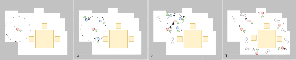
We use a guided seeded random sampling approach to initialize our viewpoints. We begin by taking a point inside the scene mesh. Then at each iteration we find the distance to the closes mesh face, define a collider and then perturb the camera pose inside that “safety sphere”. We define this as,

r_t = \min_{f \in \mathcal{F}} \operatorname{dist}(\mathbf{c}_t, f)

This process is followed by culling where we remove degenerate camera poses using semantic diversity in the scene. Finally, we run this for 100 iterations to sample 50 valid candidate poses.

\tilde{\mathbf{c}}_t = \mathbf{c}_t + \boldsymbol{\epsilon}, \quad \boldsymbol{\epsilon} \sim \mathcal{U}\big(\{\boldsymbol{x} \in \mathbb{R}^3 : \|\boldsymbol{x}\|_2 \le r_t\}\big).

\tilde{R}_t = R_{\text{t-1}} \, \delta R_.

The culling is defined as,

\theta_t = \cos^{-1}(\mathbf{v}_t^\top \mathbf{d}_t) > \tau_{deg}

Current Approach

Beyond the baselines that we have sampled, our current approach is straightforward. Here, we use a differentiable rendering pipeline to optimize the camera pose based on the z-buffer depth prediction.

Instead of conventional pixel-wise regression losses such as $\ell_1$ or $\ell_2$ , we incorporate a patch-wise ordinal loss into the objective function. The motivation for this design choice is that our primary concern is not strict numerical accuracy of depth values on an absolute scale, but rather the preservation of relative depth relationships and the avoidance of distributional inconsistencies (e.g., incorrect foreground–background ordering).

Instead of enforcing point-wise agreement, the patch-wise formulation evaluates depth relationships over local regions, encouraging consistent ordinal structure within each patch. This makes the loss more robust to global scale and shift ambiguities that commonly arise in monocular depth estimation. By operating at the patch level, the loss captures local geometric context and penalizes violations of relative depth ordering that are perceptually significant but may be weakly reflected in pixel-wise metrics.

Our final objective function is therefore defined as follows:

\Delta g = \mathcal{D}_{R, \delta}(i) – \mathcal{D}_{R, \delta}(j), \qquad \Delta p = \hat{\mathcal{D}}_{R, \delta}(i) – \hat{\mathcal{D}}_{R, \delta}(j),

\mathcal{L}_{>} = \log(1 + e^{-\Delta p}), \quad \mathcal{L}_{<} = \log(1 + e^{\Delta p}), \quad \mathcal{L}_{=} = |\Delta p|.

Then the overall patchwise loss is given as,

\mathcal{L}_{\text{patch}}^{(n)} = \frac{ \mathcal{L}_{>}^{(n)} + \mathcal{L}_{<}^{(n)} + \mathcal{L}_{=}^{(n)} }{ M }.

On top of the patchwise loss, we also define a collision regularization term,

d = \min_{f \in \mathcal{F}} \operatorname{dist}(\delta, f),

\mathcal{L}_{dist} = \max(0, d_{th} – d)^2

Giving us the final loss defined as,

\mathcal{L}_{depth} = \max_{R, \delta} \lambda_{ord} \mathcal{L}_{ordinal} + \min_{R, \delta} \lambda_{dist} \mathcal{L}_{dist},

Overall, this approach combines the advantages of various approaches as shown below.

Metrics

To quantitatively assess the accuracy of predicted depth maps, we use commonly adopted metrics in monocular depth estimation that capture both relative and absolute errors.

1. Absolute Relative Error (AbsRel). $\text{AbsRel} = \frac{1}{N} \sum_{i=1}^{N} \frac{|d_i – d_i^*|}{d_i^*}$ where $d_i$ and $d_i^*$ are the predicted and ground-truth depth values for pixel $i$ i, and $N$ is the number of valid pixels. AbsRel measures the fractional error relative to the true depth, highlighting overall magnitude discrepancies.

2. Accuracy under Threshold.

We specifically use the delta1 scores.

\delta_n = \frac{\text{num of pixels such that } \max \Big(\frac{d_i}{d_i^*}, \frac{d_i^*}{d_i}\Big) < 1.25^n}{N}

This metric evaluates the percentage of pixels where the predicted depth is within a multiplicative factor $1.25^n$ of the ground truth. Common choices are $n = 1, 2, 3$ capturing increasingly relaxed tolerances. Higher $\delta_n$ indicates better depth alignment.

3. Interpretation.

Lower AbsRel indicates closer absolute agreement with ground truth depth values.

Higher $\delta_1$ indicates better relative ordering and consistency of depth predictions.

These metrics together provide a balanced view of depth prediction quality: AbsRel captures absolute scale errors, while $\delta_1$ captures relative depth consistency, which is particularly relevant when evaluating robustness to adversarial viewpoints or across different camera configurations.