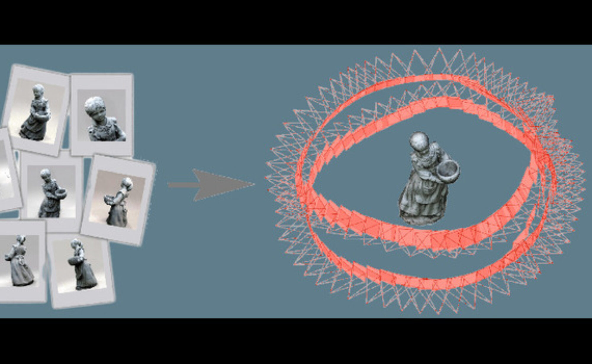
Our method works with as few as 4 input images without camera pose information to directly predict 3D Gaussians’ attributes that can then be rendered from any novel view using rasterization. It also predicts camera rays supervised on ground-truth camera pose information. The following steps outline our approach:
- Data preprocessing:
- Rescale each scene so that each view is within a certain distance (unit distance) from the object of interest. We use triangulation to find the point of intersection of all cameras’ optical axes and use this to perform the rescaling.
- Randomly select one of the camera frames as the world frame and redefine all information (camera information if available) w.r.t. to this selected world frame so that this selected camera’s center is now the world origin and the camera has identity rotation.
- Feature Extraction:
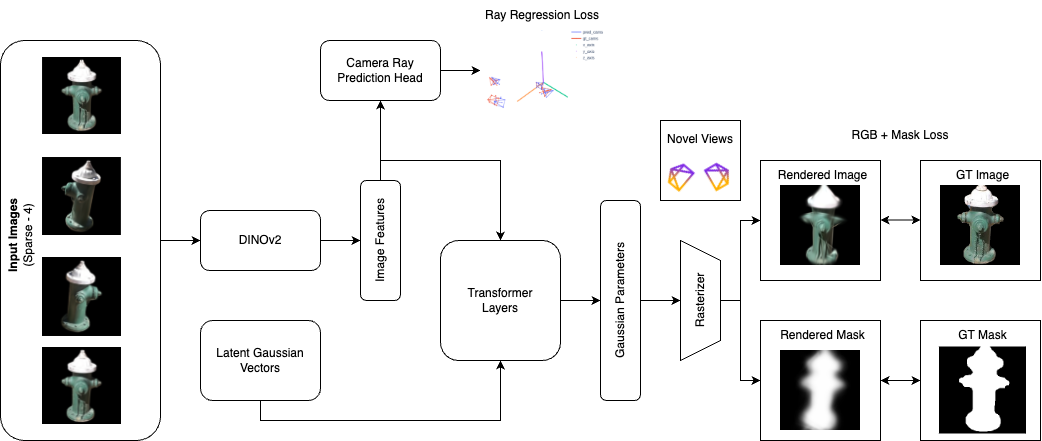
- We use the pre-trained DINOv2 model to extract patch-level features for all input images.
- We concatenate sinusoidal image positional embeddings to differentiate the first view (which is considered the world frame) from the rest.
- We concatenate patch-level sinusoidal positional embeddings similar to ViT to differentiate between different patches within each input image.
- If camera information is available in the form of a projection matrix (a combination of intrinsic and extrinsic information), we concatenate sinusoidal positional embeddings of these matrices for each image.
- We pass the final patch-level features of all images through a self-attention layer to implicitly find correspondences across images and share multi-view information.
- Transformer Blocks:
- We randomly initialize a set of latent vectors where each vector is used to predict K Gaussians towards the end of the pipeline.
- These latent vectors and the previously extracted input images’ features are passed through several transformer blocks consisting of self-attention and cross-attention layers to adequately condition the latent Gaussian vectors for the final predictions.
- Similar to the above transformer blocks there are a few self-attention transformer blocks that take in image features and predict the camera pose as rays.
- Rendering:
- In the end, we pass the latent Gaussian vectors through a linear layer followed by appropriate activation functions to predict the respective Gaussian attributes of opacity, scale, rotation, means, and RGB. These Gaussians are defined w.r.t. the first view’s frame.
- We use the rasterizer from vanilla 3DGS to render these predicted Gaussians from a given view.
- Loss:
- We apply an initialization loss directly on the predicted Gaussians’ means and scales for about 1.5k iterations to make sure the network has a good initialization.
- After this phase, we apply an RGB loss (MSE) on the renderings obtained from the predicted Gaussians. We use the 4 input views and 2 additional unseen views for this loss.
- During the above phase, a parallel branch takes in the image features and predicts camera rays and an MSE loss is applied between the predicted rays and GT rays.
- Inference: Once trained on a large-scale dataset, our pipeline just needs to be fed a few input images (as few as 4) to predict a 3D representation in the form of 3D Gaussians in a single feed-forward pass without any scene-specific optimization, unlike vanilla 3DGS. We also predict camera rays in parallel which are then used to further refine the output fidelity using test-time adaptation.