Problem Statement
Grasping and manipulating transparent objects poses a significant challenge for robots. Recent work showed neural radiance fields (NeRFs) work well for depth perception in scenes with transparent objects, and these depth maps can be used to grasp transparent objects with high accuracy. NeRF- based depth reconstruction can still struggle with challenging transparent objects and lighting conditions. In this work, we study the performance of Gaussian Splatting (3DGS) for depth perception of transparent objects.
We propose two methods, Clear-Splatting [43] and ClearSplatting-2.0.
Clear- Splatting: ⭐️ Spotlight Presentation at RoboNeRF workshop at ICRA-2024
We first train vanilla 3D Gaussian Splatting (3DGS) on our synthetic blender dataset consisting of transparent objects on a table-top setting. In order to train a 3DGS we need a multi-view dataset and the output from the algorithm is a point cloud. This point cloud is an explicit representation that can be very useful for downstream tasks since it is easy to manipulate an explicit representation such as a point cloud.


Fig5. 3D Gaussian Splatting base algorithm


Fig6. Outputs from baseline 3D Gaussian Splatting
From figures 5 and 6 we can see that the geometry learnt by 3DGS is highly plagued with floaters. These floaters are not only visible in the point cloud but also in the depth rendering in figure 6. Since 3DGS is optimized in RGB domain, hence, the RGB rendering looks fine visually but the flaw in the geometry is brought out in the depth maps.
Proposed Approach
Learning Residual Splats
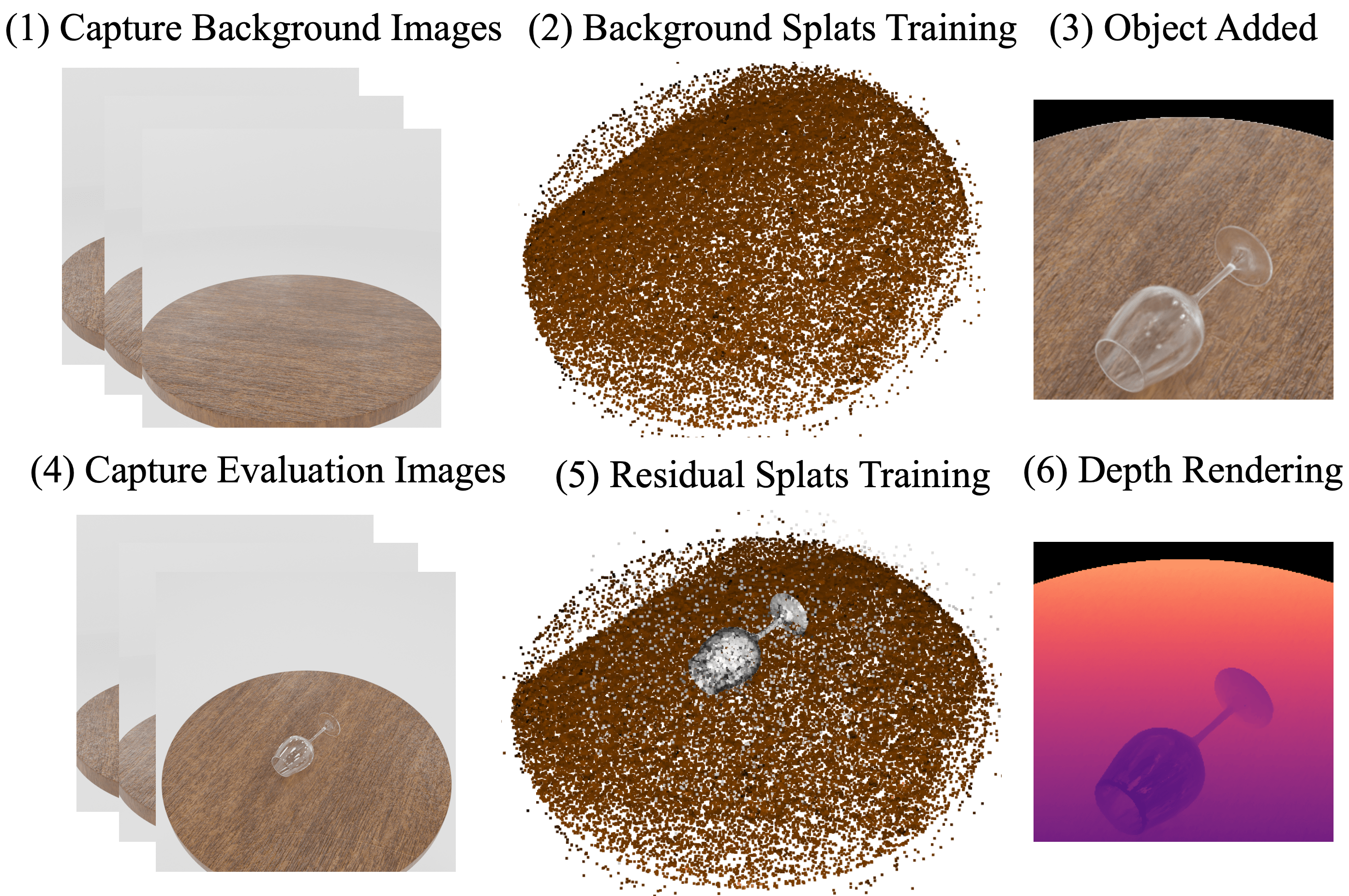
Clear-Splatting first initializes Gaussians in random states and optimizes for view reconstruction to find background Splats of the environment without the transparent object present. We then reset the optimizer and introduce a new smaller set of residual Gaussians, and optimize the state of all Gaussians simultaneously. The background Gaussians are not frozen to facilitate learning of visual effects introduced by the added object, such as shadow and reflections.
Depth from Gaussian Splatting
For Clear-Splatting, we adopt an approach inspired by Ichnowski et al. [1] and Luiten et al. [39]. We set the per- pixel depth as the depth of the Gaussian center where the accumulated transmittance of the ray drops below a threshold ‘m‘. If a ray does not reach this threshold it is assigned a high default depth. This method of calculating depth avoids perceiving floaters around depth boundaries compared to alpha-blending the depths of the Gaussians. We use m = 0.7 in our experiments, obtained empirically.
Depth based Gaussian pruning
In addition, we also introduce depth pruning where we prune the Gaussians that are within a threshold d distance in a given view, at a set frequency of training iterations and lasts until Gaussian densification [10] happens to help the remaining Gaussians adjust the learnt features. This is instrumental in dealing with occlusions in the depth domain, resulting primarily from floaters which are sets of unoptimized Gaussians that persist due to textureless background in the training views.
Figure 8 shows the final learnt geometry represented as point cloud. In comparison to figure 5 we see that the point cloud is much more defined and hence, leads to better depth estimation.

ClearSplatting-2.0: Using imperfect world models for depth distillation
A major assumption of Clear-Splatting was the presence of background images in isolation, i.e, without the transparent object in the scene. Learning the background scene was a way to introduce priors which led to a better geometry capture for the transparent objects when added subsequently into the background scene. However, this was also a limitation of the method since we might not always have the background-only images available. To overcome this limitation, we propose the use of ‘world’ models for injecting priors while modeling the 3D scene.
Since we tackle the task of metric depth estimation, we propose to use monocular depth estimators. However, depth estimators tend to fail for transparent objects. Amongst all the monocular depth estimators that we tested, Depth Anything V2 [42] resulted in the best performance for transparent objects. However, even Depth Anything V2 had its limitations, as shown in figure 9.


Fig9. Failure case of Depth Anything V2 on transparent object
Even though monocular depth estimators fail on transparent objects, they are excellent tools for distilling world priors while 3D modelling the scene. We come up with a novel approach to distill information from them while staying robust to the imperfections. We break the training into two stages, 1) using the monocular depth estimator in-distribution, and 2) using it out-of-distribution.
Stage 1
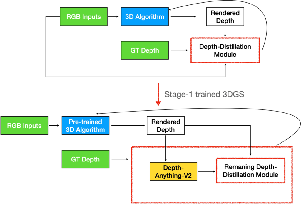
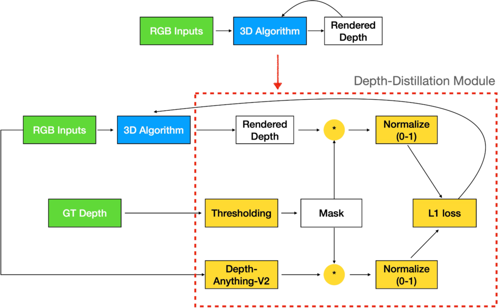
We train the 3DGS algorithm with depth supervision. The RGB images are fed to the Depth Anything V2 (DAV2) model to obtain an approximation of the ground truth depth. Since the depth obtained from monocular depth estimators have scale shift, we normalize the output of DAV2 and also normalize the rendered depth from 3DGS. We calculate the L1 loss between the normalized values to perform depth supervision for stage 1 training as shown in figure 10.
Stage 2
Simply executing stage 1 is not enough since the depth maps obtained from DAV2 are imperfect, as demonstrated in figure 9. Hence, we also perform stage 2 training.
In stage 2, we operate DAV2 with out-of-distribution data. Instead of feedig RGB training images to DAV2, we render depth from the stage 1 trained 3DGS and feed them to DAV2 to obtain the monocular depth maps, as shown in figure 11.
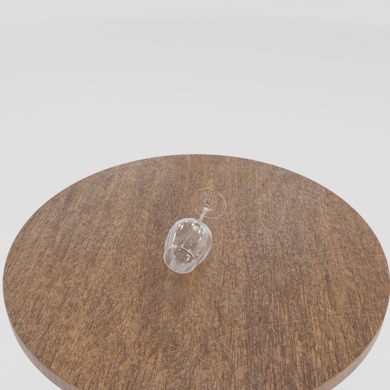
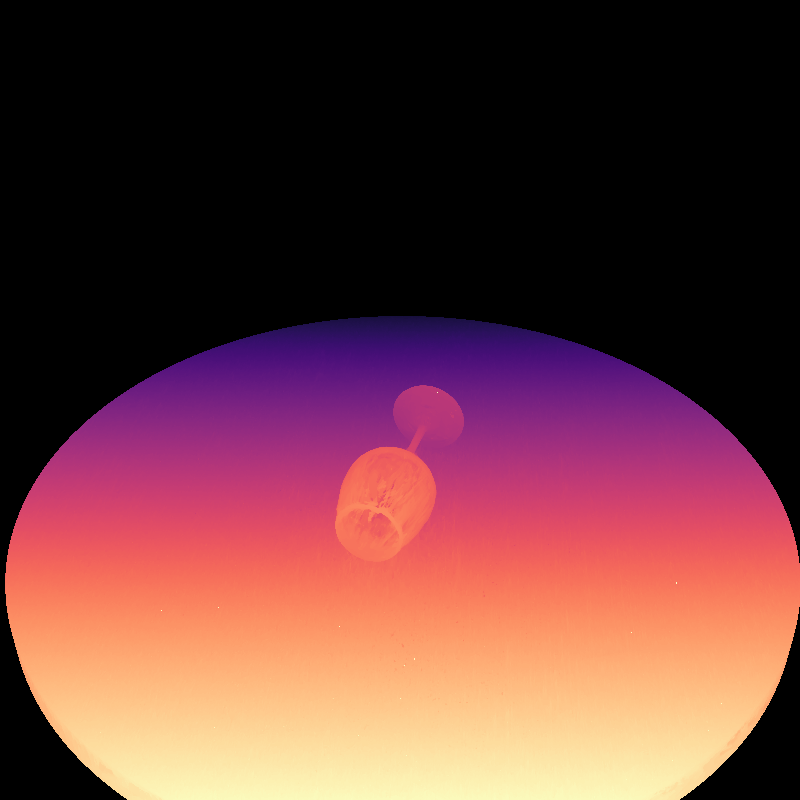

Fig11. Depth Anything V2 output given 3DGS rendered depth as input
From figure 11 we see that DAV2 is now able to generate correct depth for the wine glass (upto a scale) in contrast to figure 9. Thus, we now use this output from DAV2 as the ground truth depth and perform the depth supervision similar to stage 1.